TensorFlow实战-从梯度下降到Mnist数据集的CNN训练
本文的基本结构:
1. 基于梯度下降的线性回归
2. Mnist数据集的逻辑回归
3. Mnist数据集的神经网络
4. Mnist数据集的卷积神经网络
5. 总结
1. 基于梯度下降的线性回归
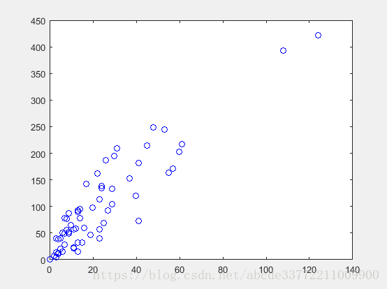
1.1 任务:给定一组数,X与Y,采用线性函数去拟合和预测
1.2 问题建模
线性实现最优拟合,自然想到通过最小化误差的最优化数学模型,假定最优化线性函数为y=ax+b,最优化问题求解:

这是一个凸优化问题,可以利用导数求解和梯度下降两种方法:
1)导数求解
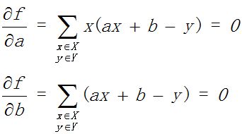 求得闭环解
求得闭环解
2)梯度下降迭代求解
a b step给一个初始值
For 迭代次数

1.3 求解实现Matlab
%样本
%Sample = rand(2,10);
%Sample = [1400 1600 1700 1875 1100 1550 2350 2450 1425 1700;245000 312000 279000 308000 199000 219000 405000 324000 319000 255000]./1000;

x = [108.0 , 19.0 , 13.0 , 124.0 , 40.0 , 57.0 , 23.0 , 14.0 , 45.0 , 10.0 , 5.0 , 48.0 , 11.0 , 23.0 , 7.0 , 2.0 , 24.0 , 6.0 , 3.0 , 23.0 , 6.0 , 9.0 , 9.0 , 3.0 , 29.0 , 7.0 , 4.0 , 20.0 , 7.0 , 4.0 , 0.0 , 25.0 , 6.0 , 5.0 , 22.0 , 11.0 , 61.0 , 12.0 , 4.0 , 16.0 , 13.0 , 60.0 , 41.0 , 37.0 , 55.0 , 41.0 , 11.0 , 27.0 , 8.0 , 3.0 , 17.0 , 13.0 , 13.0 , 15.0 , 8.0 , 29.0 , 30.0 , 24.0 , 9.0 , 31.0 , 14.0 , 53.0 , 26.0 ];
y = [392.5 , 46.2 , 15.7 , 422.2 , 119.4 , 170.9 , 56.9 , 77.5 , 214.0 , 65.3 , 20.9 , 248.1 , 23.5 , 39.6 , 48.8 , 6.6 , 134.9 , 50.9 , 4.4 , 113.0 , 14.8 , 48.7 , 52.1 , 13.2 , 103.9 , 77.5 , 11.8 , 98.1 , 27.9 , 38.1 , 0.0 , 69.2 , 14.6 , 40.3 , 161.5 , 57.2 , 217.6 , 58.1 , 12.6 , 59.6 , 89.9 , 202.4 , 181.3 , 152.8 , 162.8 , 73.4 , 21.3 , 92.6 , 76.1 , 39.9 , 142.1 , 93.0 , 31.9 , 32.1 , 55.6 , 133.3 , 194.5 , 137.9 , 87.4 , 209.8 , 95.5 , 244.6 , 187.5];
Len = length(x);

%变量初始化Para为a b迭代数组,delta De为迭代过程中的误差,f为目标函数值
Para = [0 0];
delta = 2;
De = [];
f = 0;
step = 0.0000001;
%梯度下降迭代
while  delta>0.001
    De = [De delta];
    dao1 = sum((Para(1)*x+Para(2)-y).*x);
    dao2 = sum((Para(1)*x+Para(2)-y));
    Para(1) = Para(1) - step*dao1;
    Para(2) = Para(2) - step*dao2;
    delta = abs(sum((Para(1).*x+ Para(2)-y).^2)/2 - f);
    f = sum((Para(1).*x+ Para(2)-y).^2)/2;
end
z = Para(1)*x + Para(2);
Para

%闭环解
a = (Len*sum(x.*y)-sum(x)*sum(y))/(Len*sum(x.^2)-sum(x)^2)
b = (sum(y)-a*sum(x))/Len

figure(1)
plot(x,y,'bo',x,a*x+b,'-',x,z,'*');
legend('样点','闭环解','梯度下降解');
figure(2);
plot(1:10,De(1:10));
legend('迭代收敛误差');

梯度解:Para =3.4206 19.6806
闭环解:a =3.4138 b =19.9945
从结果看,闭环解和梯度下降解一致,误差收敛速度10次基本已收敛。

1.3 梯度求解技巧
在梯度下降的求解过程中,发现a b的初始值,训练步长对于收敛产生重要影响。
1) a b初始值影响
a b的初始值对于收敛速率有一定影响,如果初值设为1000 1000,收敛结果如下,但是不至于不能收敛。

2) 调整步长的影响
调整步长设置不合适,有可能会错过最优点,造成不能收敛,如设置为0.001,就不能收敛,变量内存溢出NaN。
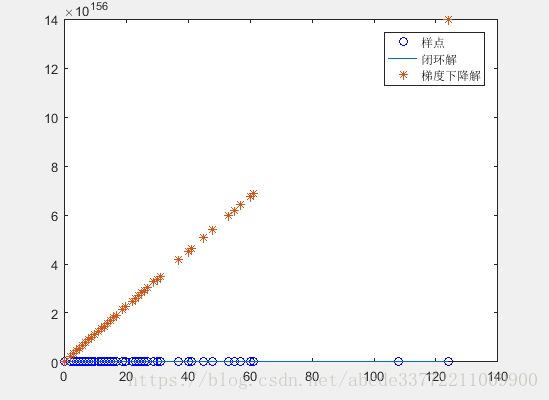
从前面公式看,步长和梯度共同影响调整的快慢和幅值,上图中原因是梯度太大导致调整太大,而步长没有降低梯度的幅值。
1.4 基于TensorFlow的线性回归实现
## 线性回归算法

import numpy as np
import tensorflow as tf
import matplotlib.pyplot as plt

# 随机生成1000个点,y=0.1x+0.3
num_points = 1000
vectors_set = []
for i in range(num_points):
    x1 = np.random.normal(0.0,0.55)
    y1 = x1 * 0.1 + 0.3 + np.random.normal(0.0,0.03)
    vectors_set.append([x1,y1])

# 样本点赋值
x_data = [v[0] for v in vectors_set]
y_data = [v[1] for v in vectors_set]
plt.scatter(x_data,y_data,c='r')
plt.show()

# 变量定义
W = tf.Variable(tf.random_uniform([1],-1,1),name='W')
b = tf.Variable(tf.constant(10.0))
y = W * x_data + b

# 目标函数
loss = tf.reduce_mean(tf.square(y - y_data))
optimizer = tf.train.GradientDescentOptimizer(0.5)
train = optimizer.minimize(loss)

#创建运行session
sess = tf.Session()
init = tf.global_variables_initializer()
sess.run(init)

print("W =",sess.run(W),"b =",sess.run(b),"loss =",sess.run(loss))
#执行梯度训练
for step in range(20):
    sess.run(train)
    print("W =",sess.run(W),"b =",sess.run(b),"loss =",sess.run(loss))

plt.scatter(x_data,y_data,c='r')
plt.plot(x_data,sess.run(W)*x_data+sess.run(b))
plt.show()
2. Mnist数据集的逻辑回归
从上面梯度下降的实现中,我们可以看到,其实是在自变量范围内,选取一个初始点,按照梯度反方向进行搜索极值点,调整步长对搜索过程也非常重要,不合适的步长会导致错过了极值点。
2.1 Mnist数据集说明
Mnist数据集,是手写数字图片,由大牛Yann leCun创建,用于进行数字识别,详细可以参考如下网址。
在导入Mnist数据集时,mnist = input_data.read_data_sets("data/", one_hot=True)在导入tensorflow自带的Mnist数据时,会发生IO错误,不能够导入数据,可能是没有包含数据包,这时可以到如下网址,将图片压缩包导入data文件夹里,就能够解决。http://yann.lecun.com/exdb/mnist/

2.2 任务
每个Mnist图像为黑白图像,大小为28*28*1,利用回归去拟合训练样本,y = WX + B。不同于上面二维线性回归,X和y都是一维,但是原理是类似,利用一个大小为10的概率向量来表示y,如,数字图片5,标签为[0 0 0 0 0 0 0 0 0 0],那么拟合最优化问题为:

其中,W大小为 10*784,B大小为10*1,X大小为784*1,y大小为10*1,
softmax函数为一个归一化概率分布,指数占比率。

由于上面最优化问题没有闭环解,所以采用梯度下降法求解。
2.3 Mnist数据逻辑回归梯度下降求解
## Mnist数据集的逻辑回归

# 工具类的简写
import numpy as np
import tensorflow as tf
import matplotlib.pyplot as plt

# 导入Mnist数据集,并且读入数据到变量Mnist,如果无法导入可参考上述说明
from tensorflow.examples.tutorials.mnist import input_data
mnist = input_data.read_data_sets("data/", one_hot=True)
print (" 类型是 %s" % (type(mnist)))
print (" 训练数据 %d" % (mnist.train.num_examples))
print (" 测试数据 %d" % (mnist.test.num_examples))

# minist变量存储的是已经定义好数据结构的Mnist数据结构
trainimg   = mnist.train.images
trainlabel = mnist.train.labels
testimg    = mnist.test.images
testlabel  = mnist.test.labels
print (" 数据类型 is %s"    % (type(trainimg)))
print (" 标签类型 %s"  % (type(trainlabel)))
print (" 训练集的shape %s"   % (trainimg.shape,))
print (" 训练集的标签的shape %s" % (trainlabel.shape,))
print (" 测试集的shape' is %s"    % (testimg.shape,))
print (" 测试集的标签的shape %s"  % (testlabel.shape,))

# 从训练数据中随机打印几张手写数字图像
nsample = 6
randidx = np.random.randint(trainimg.shape[0], size=nsample)
for i in randidx:
    curr_img   = np.reshape(trainimg[i, :], (28, 28))     # 28 by 28 matrix
    curr_label = np.argmax(trainlabel[i, :])              # Label
    plt.matshow(curr_img, cmap=plt.get_cmap('gray'))
    print ("" + str(i) + "th 训练数据 "
           + "标签是 " + str(curr_label))
    plt.show()

# 对数据进行打包,Batch数据
batch_size = 100
batch_xs, batch_ys = mnist.train.next_batch(batch_size)
print ("Batch数据 %s" % (type(batch_xs)))
print ("Batch标签 %s" % (type(batch_ys)))
print ("Batch数据的shape %s" % (batch_xs.shape,))
print ("Batch标签的shape %s" % (batch_ys.shape,))

# 设置模型参数
numClasses = 10
inputSize = 784
trainingIterations = 50000
batchSize = 64

# 变量的定义
    # placeholder数据类型
X = tf.placeholder(tf.float32,shape = [None, inputSize])
y = tf.placeholder(tf.float32,shape = [None, numClasses])
# 需要求解的权值参数y = W1*X + B1
    # W1服从正态分布784*10 B1常数1*10
W1 = tf.Variable(tf.random_normal([inputSize, numClasses], stddev=0.1))
B1 = tf.Variable(tf.constant(0.1),[numClasses])

# 优化的目标函数,监测变量的定义
    # y = W1*X + B1 ---softmax函数
y_pred = tf.nn.softmax(tf.matmul(X,W1) + B1)  # 10*1的概率分布
loss = tf.reduce_mean(tf.square(y - y_pred))
opt = tf.train.GradientDescentOptimizer(learning_rate= 0.05).minimize(loss)
correct_prediction = tf.equal(tf.argmax(y_pred,1), tf.argmax(y,1))
accuracy = tf.reduce_mean(tf.cast(correct_prediction, "float"))

# 工作环境初始化
sess = tf.Session()
init = tf.global_variables_initializer()
sess.run(init)

# 梯度下降的迭代
for i in range(trainingIterations):
    batch = mnist.train.next_batch(batchSize)
    batchInput = batch[0]
    batchLabels = batch[1]     #数据分批完成读入并且赋值
    # 梯度下降求解一次
    trainingLoss = sess.run([opt, loss], feed_dict={X: batchInput, y: batchLabels})
    # 每累计求解1000次,查看训练结果
    if i%1000 == 0:
        train_accuracy = accuracy.eval(session=sess, feed_dict={X: batchInput, y: batchLabels})
        print ("step %d, training accuracy %g"%(i, train_accuracy))

# 循环完成后,模型参数训练完成W1 B1,利用测试数据进行验证
batch = mnist.test.next_batch(batchSize)
testAccuracy = sess.run(accuracy, feed_dict={X: batch[0], y: batch[1]})
print ("test accuracy %g"%(testAccuracy))
3. Mnist数据集的神经网络
在2中,我们采用回归拟合思路,利用梯度下降方法,求解得到拟合函数的参数,达到识别目的;由于拟合思想还是基于训练样本误差最小化,所以过拟合风险较大,并没有提取到每一类别的关键特征,泛化能力不强,有没有一种结构或机制,能够提取到某类别最独特的信息,达到高准确识别和强泛化,神经网络给出了答案。
神经网络通过隐藏层的引入,对信息提取进行门限筛选,过滤掉了影响不大的信息,通过激活函数来实现。
下面分别用一层隐藏层,两次隐藏层进行实现。
# Mnist数据集 神经网络实现

import tensorflow as tf
from tensorflow.examples.tutorials.mnist import input_data
mnist = input_data.read_data_sets("data/", one_hot=True)

# 设置网络参数
numClasses = 10
inputSize = 784
numHiddenUnits = 50     # 隐藏单元50个
trainingIterations = 10000
batchSize = 100

# 变量定义
X = tf.placeholder(tf.float32, shape = [None, inputSize])
y = tf.placeholder(tf.float32, shape = [None, numClasses])
W1 = tf.Variable(tf.truncated_normal([inputSize, numHiddenUnits], stddev=0.1))
B1 = tf.Variable(tf.constant(0.1), [numHiddenUnits])
W2 = tf.Variable(tf.truncated_normal([numHiddenUnits, numClasses], stddev=0.1))
B2 = tf.Variable(tf.constant(0.1), [numClasses])

# 网络结构搭建
hiddenLayerOutput = tf.matmul(X, W1) + B1
hiddenLayerOutput = tf.nn.relu(hiddenLayerOutput)
finalOutput = tf.matmul(hiddenLayerOutput, W2) + B2
finalOutput = tf.nn.relu(finalOutput)

# 目标函数
loss = tf.reduce_mean(tf.nn.softmax_cross_entropy_with_logits(labels = y, logits = finalOutput))
opt = tf.train.GradientDescentOptimizer(learning_rate = .1).minimize(loss)
correct_prediction = tf.equal(tf.argmax(finalOutput,1), tf.argmax(y,1))
accuracy = tf.reduce_mean(tf.cast(correct_prediction, "float"))

# 运行会话
sess = tf.Session()
init = tf.global_variables_initializer()
sess.run(init)

# 梯度下降求解
for i in range(trainingIterations):
    batch = mnist.train.next_batch(batchSize)
    batchInput = batch[0]
    batchLabels = batch[1]
    _, trainingLoss = sess.run([opt, loss], feed_dict={X: batchInput, y: batchLabels})
    if i%1000 == 0:
        trainAccuracy = accuracy.eval(session=sess, feed_dict={X: batchInput, y: batchLabels})
        print ("step %d, training accuracy %g"%(i, trainAccuracy))

## 两层隐藏层引入

# 参数设定
numHiddenUnitsLayer2 = 100
trainingIterations = 10000

# 变量定义
X = tf.placeholder(tf.float32, shape = [None, inputSize])
y = tf.placeholder(tf.float32, shape = [None, numClasses])
W1 = tf.Variable(tf.random_normal([inputSize, numHiddenUnits], stddev=0.1))
B1 = tf.Variable(tf.constant(0.1), [numHiddenUnits])
W2 = tf.Variable(tf.random_normal([numHiddenUnits, numHiddenUnitsLayer2], stddev=0.1))
B2 = tf.Variable(tf.constant(0.1), [numHiddenUnitsLayer2])
W3 = tf.Variable(tf.random_normal([numHiddenUnitsLayer2, numClasses], stddev=0.1))
B3 = tf.Variable(tf.constant(0.1), [numClasses])

# 网络结构
hiddenLayerOutput = tf.matmul(X, W1) + B1
hiddenLayerOutput = tf.nn.relu(hiddenLayerOutput)
hiddenLayer2Output = tf.matmul(hiddenLayerOutput, W2) + B2
hiddenLayer2Output = tf.nn.relu(hiddenLayer2Output)
finalOutput = tf.matmul(hiddenLayer2Output, W3) + B3

# 目标函数
    # tf.nn.softmax和tf.nn.softmax_cross_entropy_with_logits差别在于有无交叉熵
loss = tf.reduce_mean(tf.nn.softmax_cross_entropy_with_logits(labels = y, logits = finalOutput))
opt = tf.train.GradientDescentOptimizer(learning_rate = .1).minimize(loss)
correct_prediction = tf.equal(tf.argmax(finalOutput,1), tf.argmax(y,1))
accuracy = tf.reduce_mean(tf.cast(correct_prediction, "float"))

# 运行会话
sess = tf.Session()
init = tf.global_variables_initializer()
sess.run(init)

# 梯度下降求解
for i in range(trainingIterations):
    batch = mnist.train.next_batch(batchSize)
    batchInput = batch[0]
    batchLabels = batch[1]
    _, trainingLoss = sess.run([opt, loss], feed_dict={X: batchInput, y: batchLabels})
    if i%1000 == 0:
        train_accuracy = accuracy.eval(session=sess, feed_dict={X: batchInput, y: batchLabels})
        print ("step %d, training accuracy %g"%(i, train_accuracy))

# 测试集验证
testInputs = mnist.test.images
testLabels = mnist.test.labels
acc = accuracy.eval(session=sess, feed_dict = {X: testInputs, y: testLabels})
print("testing accuracy: {}".format(acc))
4. Mnist数据集的卷积神经网络CNN
在3中,我们采用神经网络模型进行识别训练,核心是加入了隐藏层,对特征强度进行筛选,接下来进一步增强识别模型的识别能力,在特征提取上,采用卷积神经网络CNN,对原始图像进行预处理,将特征信息进行增强。
对于Mnist数据集识别所构建的神经网络结构如下,从图中可以发现,第一层卷积有32个卷积单元,第二层卷积有64个卷积单元,每一层卷积后进行最大池化将图像大小缩小为原来的一半,第一层全连接层,将64个7*7的矩阵级联转化为大小为1024向量,第二层全连接,将大小为1024向量转化为大小为10向量,除了最后一层全连接层没有使用激活函数,两个卷积层和一个全连接层都使用了激活函数。
网络结构如下,其中Conv(k1,N1,1)代表卷积层输入为1个单元,输出为N1个单元,卷积核大小为k1*k1;Maxpool(2)为最大池化,将图像大小缩小一倍;FC(1024)为全连接层,大小为1024向量。

## Mnist数据集采用CNN网络结构进行识别
import tensorflow as tf
import random
import numpy as np
import matplotlib.pyplot as plt
import datetime
%matplotlib inline

# 导入数据
from tensorflow.examples.tutorials.mnist import input_data
mnist = input_data.read_data_sets("data/", one_hot=True)

tf.reset_default_graph()
sess = tf.InteractiveSession()

# 变量定义
x = tf.placeholder("float", shape = [None, 28,28,1])                 #shape in CNNs is always None x height x width x color channels
y_ = tf.placeholder("float", shape = [None, 10])                     #shape is always None x number of classes

# 第一个卷积层和池化操作
W_conv1 = tf.Variable(tf.truncated_normal([5, 5, 1, 32], stddev=0.1))#shape is filter x filter x input channels x output channels
b_conv1 = tf.Variable(tf.constant(.1, shape = [32]))                 #shape of the bias just has to match output channels of the filter
h_conv1 = tf.nn.conv2d(input=x, filter=W_conv1, strides=[1, 1, 1, 1], padding='SAME') + b_conv1
h_conv1 = tf.nn.relu(h_conv1)
h_pool1 = tf.nn.max_pool(h_conv1, ksize=[1, 2, 2, 1], strides=[1, 2, 2, 1], padding='SAME')

def conv2d(x, W):
    return tf.nn.conv2d(input=x, filter=W, strides=[1, 1, 1, 1], padding='SAME')
def max_pool_2x2(x):
    return tf.nn.max_pool(x, ksize=[1, 2, 2, 1], strides=[1, 2, 2, 1], padding='SAME')

# 第二个卷积层和池化操作
W_conv2 = tf.Variable(tf.truncated_normal([5, 5, 32, 64], stddev=0.1))
b_conv2 = tf.Variable(tf.constant(.1, shape = [64]))
h_conv2 = tf.nn.relu(conv2d(h_pool1, W_conv2) + b_conv2)
h_pool2 = max_pool_2x2(h_conv2)

# 第一个全连接层,将64个7*7图像数据,级联成7*7*64,再转化为1024大小向量
W_fc1 = tf.Variable(tf.truncated_normal([7 * 7 * 64, 1024], stddev=0.1))
b_fc1 = tf.Variable(tf.constant(.1, shape = [1024]))
h_pool2_flat = tf.reshape(h_pool2, [-1, 7*7*64])
h_fc1 = tf.nn.relu(tf.matmul(h_pool2_flat, W_fc1) + b_fc1)

# 随机丢失层,对一些神经元随机杀死,防止训练数据的过拟合
keep_prob = tf.placeholder("float")
h_fc1_drop = tf.nn.dropout(h_fc1, keep_prob)

# 第二个全连接层,将1024大小向量转化为大小10向量
W_fc2 = tf.Variable(tf.truncated_normal([1024, 10], stddev=0.1))
b_fc2 = tf.Variable(tf.constant(.1, shape = [10]))

# 最后输出结果
y = tf.matmul(h_fc1_drop, W_fc2) + b_fc2

# 目标函数的设计
crossEntropyLoss = tf.reduce_mean(tf.nn.softmax_cross_entropy_with_logits(labels = y_, logits = y))
trainStep = tf.train.AdamOptimizer().minimize(crossEntropyLoss)
correct_prediction = tf.equal(tf.argmax(y,1), tf.argmax(y_,1))
accuracy = tf.reduce_mean(tf.cast(correct_prediction, "float"))
sess.run(tf.global_variables_initializer())

# 采用自适应矩估计最优化方法
batchSize = 50
for i in range(1000):
    batch = mnist.train.next_batch(batchSize)
    trainingInputs = batch[0].reshape([batchSize,28,28,1])
    trainingLabels = batch[1]
    if i%100 == 0:
        trainAccuracy = accuracy.eval(session=sess, feed_dict={x:trainingInputs, y_: trainingLabels, keep_prob: 1.0})
        print ("step %d, training accuracy %g"%(i, trainAccuracy))
    trainStep.run(session=sess, feed_dict={x: trainingInputs, y_: trainingLabels, keep_prob: 0.5})
5. 总结
回顾上面的过程,从二维点图线性回归到图像识别的线性回归,从线性回归的图像识别到神经网络识别,再到卷积神经网络识别,其中经历了几十年的发展过程,如今罗列出来却显得那么简单,科学的探索是严谨和艰难,假如将我们自己放之于历史过程中,是否也会对未来充满未知,对现有技术方向或坚持,或彷徨不定,但是唯有坚持探索不放弃,才能够不断开拓进步。