obspy中文教程(七)
Visualize Data Availability of Local Waveform Archive(可视化本地波形存档数据的可用性)
通常,您拥有大量数据并希望知道哪个站点在何时是可用的。对于这种假设的情况,obspy提供了obspy-scan脚本(安装后即可用),它能从文件的数据头检测文件格式(MiniSEED, SAC, SACXY, GSE2, SH-ASC, SH-Q, SEISAN, 等),在间隙处绘制为垂直红线,可用数据的在开始时间绘制十字,数据本身绘为水平线。该脚本可以扫描超过1000个文件(已有被用于扫描30000个文件,耗时约45分钟。),自动绘制年/月范围。它会打开一个可放大的交互式绘图窗口。
从命令提示符执行类似下面的语句,使用通配符匹配文件:
$ obspy-scan /bay_mobil/mobil/20090622/1081019/*_1.*
Travel Time and Ray Path Plotting(走时和射线路径绘制)
走时绘制
下面的代码展示如何plot_travel_times()函数绘制给定距离和相位的使用iasp91速度模型计算出的走时。
from obspy.taup import plot_travel_times

import matplotlib.pyplot as plt


fig, ax = plt.subplots()

ax = plot_travel_times(source_depth=10, ax=ax, fig=fig,

                       phase_list=['P', 'PP', 'S'], npoints=200)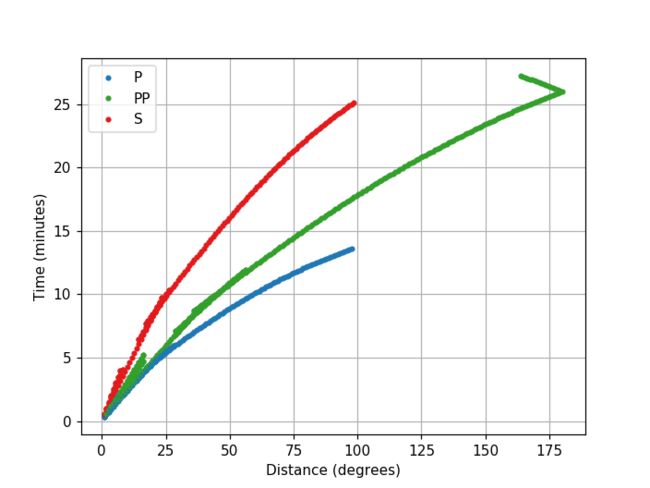
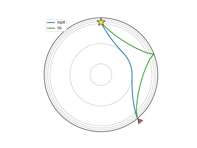
笛卡尔射线路径
下面的几行代码展示了如何绘制给定距离和相位的射线路径。射线路径使用iasp91速度模型计算,并使用obspy.taup.tau.Arrivals类的plot_rays()函数的绘制(在笛卡尔坐标系中)。
from obspy.taup import TauPyModel


model = TauPyModel(model='iasp91')

arrivals = model.get_ray_paths(500, 140, phase_list=['PP', 'SSS'])

arrivals.plot_rays(plot_type='cartesian', phase_list=['PP', 'SSS'],

                   plot_all=False, legend=True)
球形射线路径
下面的几行代码展示了如何绘制给定距离和相位的射线路径。射线路径使用iasp91速度模型计算,并使用obspy.taup.tau.Arrivals类的plot_rays()函数的绘制(在球形图中)。
多距离射线路径
下面的几行代码展示了如何绘制有多个震中距和相位的射线路径。射线路径使用iasp91速度模型计算,并使用obspy.taup.tau.Arrivals类的plot_ray_paths()函数的绘制(在球形图中)。
from obspy.taup.tau import plot_ray_paths

import matplotlib.pyplot as plt


fig, ax = plt.subplots(subplot_kw=dict(polar=True))

ax = plot_ray_paths(source_depth=100, ax=ax, fig=fig, phase_list=['P', 'PKP'],

                    npoints=25)
对于单个震中距离的射线路径示例,请尝试上一节中的plot_rays()方法。以下是一个更高级的示例,其中包含自定义的相位和距离列表:
import numpy as np

import matplotlib.pyplot as plt


from obspy.taup import TauPyModel


PHASES = [

    # Phase, distance

    ('P', 26),

    ('PP', 60),

    ('PPP', 94),

    ('PPS', 155),

    ('p', 3),

    ('pPcP', 100),

    ('PKIKP', 170),

    ('PKJKP', 194),

    ('S', 65),

    ('SP', 85),

    ('SS', 134.5),

    ('SSS', 204),

    ('p', -10),

    ('pP', -37.5),

    ('s', -3),

    ('sP', -49),

    ('ScS', -44),

    ('SKS', -82),

    ('SKKS', -120),

]


model = TauPyModel(model='iasp91')


fig, ax = plt.subplots(subplot_kw=dict(polar=True))


# Plot all pre-determined phases

for phase, distance in PHASES:

    arrivals = model.get_ray_paths(700, distance, phase_list=[phase])

    ax = arrivals.plot_rays(plot_type='spherical',

                            legend=False, label_arrivals=True,

                            plot_all=True,

                            show=False, ax=ax)


# Annotate regions

ax.text(0, 0, 'Solid\ninner\ncore',

        horizontalalignment='center', verticalalignment='center',

        bbox=dict(facecolor='white', edgecolor='none', alpha=0.7))

ocr = (model.model.radius_of_planet -

       (model.model.s_mod.v_mod.iocb_depth +

        model.model.s_mod.v_mod.cmb_depth) / 2)

ax.text(np.deg2rad(180), ocr, 'Fluid outer core',

        horizontalalignment='center',

        bbox=dict(facecolor='white', edgecolor='none', alpha=0.7))

mr = model.model.radius_of_planet - model.model.s_mod.v_mod.cmb_depth / 2

ax.text(np.deg2rad(180), mr, 'Solid mantle',

        horizontalalignment='center',

        bbox=dict(facecolor='white', edgecolor='none', alpha=0.7))


plt.show()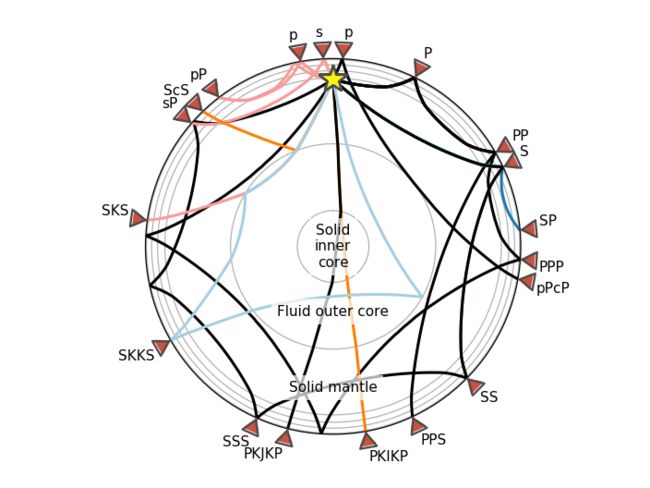
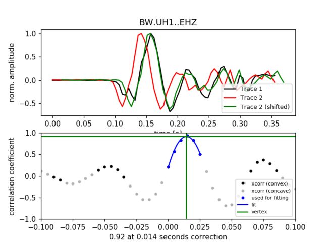
Cross Correlation Pick Correction(互相关拾取校正)
该示例展示如何对齐两个地震的起始波形相位,以便纠正在常规分析中无法完全设置一致的原始拾取时间。按照[Deichmann1992]的方法,互相关函数的凹陷部分最大值附近可用抛物线拟合。
为调整参数并验证检查结果,可以选择展示图形或者将其存为图像文件。参见xcorr_pick_correction()。
该示例将打印拾取序列2的时间校正和相应的相关系数,并打开原始和预处理数据相关性的绘图窗口:
No preprocessing:

  Time correction for pick 2: -0.014459

  Correlation coefficient: 0.92

Bandpass prefiltering:

  Time correction for pick 2: -0.013025

  Correlation coefficient: 0.98
from __future__ import print_function


import obspy

from obspy.signal.cross_correlation import xcorr_pick_correction


# read example data of two small earthquakes

path = "https://examples.obspy.org/BW.UH1..EHZ.D.2010.147.%s.slist.gz"

st1 = obspy.read(path % ("a", ))

st2 = obspy.read(path % ("b", ))

# select the single traces to use in correlation.

# to avoid artifacts from preprocessing there should be some data left and

# right of the short time window actually used in the correlation.

tr1 = st1.select(component="Z")[0]

tr2 = st2.select(component="Z")[0]

# these are the original pick times set during routine analysis

t1 = obspy.UTCDateTime("2010-05-27T16:24:33.315000Z")

t2 = obspy.UTCDateTime("2010-05-27T16:27:30.585000Z")


# estimate the time correction for pick 2 without any preprocessing and open

# a plot window to visually validate the results

dt, coeff = xcorr_pick_correction(t1, tr1, t2, tr2, 0.05, 0.2, 0.1, plot=True)

print("No preprocessing:")

print("  Time correction for pick 2: %.6f" % dt)

print("  Correlation coefficient: %.2f" % coeff)

# estimate the time correction with bandpass prefiltering

dt, coeff = xcorr_pick_correction(t1, tr1, t2, tr2, 0.05, 0.2, 0.1, plot=True,

                                  filter="bandpass",

                                  filter_options={'freqmin': 1, 'freqmax': 10})

print("Bandpass prefiltering:")

print("  Time correction for pick 2: %.6f" % dt)

print("  Correlation coefficient: %.2f" % coeff)