BB_twtr 使用CNNs+LSTMs做SemEval-2017 Task 4

paper： BB twtr at SemEval-2017 Task 4: Twitter Sentiment Analysis with CNNs and LSTMs

Abstract：
Our system leverages a large amount of unlabeled data to pre-train word embeddings.
We then use a subset of the unlabeled data to fine tune the embeddings using distant supervision.

The final CNNs and LSTMs are trained on the SemEval-2017 Twitter dataset where the embeddings are fined tuned again.

---

1 Introduction
In sec. 3 we expand on the three training phases used in our system.
In sec. 4 we discuss the various tricks that were used to fine tune the system for each individual subtasks

第三节：扩充了三个训练步骤
第四节：微调每个子任务的技巧

---

System description：

CNN

The input of the network are the tweets, which are tokenized into words
输入是被标记成单词的 tweets
Each word is mapped to a word vector representation.

an entire tweet can be mapped to a matrix of size s × d
s 有多少个词
d is the dimension of the embedding space( we chose d = 200)

所有的 tweets have the same matrix dimension X (80 * 200)

我们应用一个卷积层： h*d
h is the size of the convolution, meaning the number of words it spans.

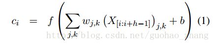
b: bias term
f(x):nonlinear function, 这里选择 relu函数

我们可以使用多个滤波矩阵来学习不同的特性，这里使用了200个滤波矩阵
We can use multiple filtering matrices to learn different features,
and additionally we can use multiple convolution sizes to focus on smaller or larger regions of the tweets.
In practice, we used three filter sizes (either [1; 2; 3], [3; 4; 5] or [5; 6; 7] depending on
the model) and we used a total of 200 filtering matrices for each filter size.

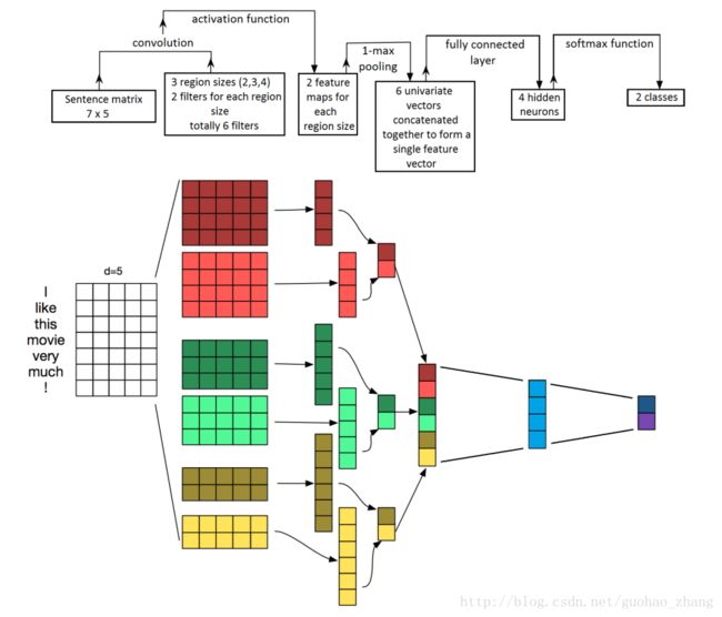
对每个卷积 max-pooling
max-pooling operation to each convolution cmax=max(c) .
作用就是
The max-pooling operation extracts the most important feature for each convolution, independently of where in the tweet this feature is located

dropout
50%（0.5）

This vector then goes through a small fully connected hidden layer of size 30
然后进入一个 fully connected hidden layer

softmax

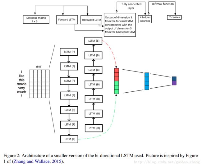
LSTM

Its main building blocks are two LSTM units.

For each element in the sequence, that is for each word in the tweet,
对于序列中的每个元素，即对于推文中的每个词，RNN使用现有的word-embeddinghe和其先前的隐藏状态来计算下一个隐藏状态

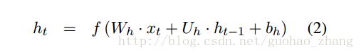
xt is the current word embedding
Wh∈R ^{m x d}
Uh∈R ^{m x m} are weight matrices,
bh∈Rm is a bias term and f(x) is a non-linear function, usually chosen to be tanh .

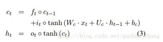
it is called the input gate,
ft is the forget gate,
ct is the cell state,
ht is the regular hidden state,
σ is the sigmoid function,
◦ is the Hadamard product.
LSTM的一个缺点是它没有充分考虑到单词信息，因为句子只能读到一个方向; forward。 为了解决这个问题，我们使用双向的LSTM，bidirectional LSTM

two LSTMs whose outputs are stacked together. One LSTM reads the sentence forward, and the other LSTM reads it backward.

在它们处理完各自的最后一个word后，我们连接每个LSTM的隐藏状态。形成了一个 2m=400的矢量

fed to a fully connected hidden layer of size 30

softmax

we add a dropout layer before and after the LSTMs, and after the fully connected
hidden layer, with a dropout probability of 50% during training.
dropout 0.5

Training

数据：
49,693 human labeled tweets for subtask A,
30,849 tweets for subtasks (C, E)
18,948 tweets for subtasks (B, D).

In addition to this human labeled data, we collected 100 million unique unlabeled English tweets using the Twitter streaming API.
从这个未标记的数据集中，我们提取了500万个正面推文和500万个负面推文

然后简单地将积极的推特与积极的表情符号（例如“:)”）相关联，反之亦然。

Those three datasets (unlabeled, distant and labeled) were used separately in the three training stages which we now present.
这三个数据集（unlabeled, distant and labeled）分别在我们现在提出的三个训练阶段中使用。
训练过程像 (Severyn and Moschitti, 2015; Deriu et al.,2016).中说到类似

Pre-processing

去网址，加颜文字关联，去重复字符，全转换小写

Unsupervised training

Google’s Word2vec (Mikolov et al.,2013a,b),
Facebook’s FastText (Bojanowski et al., 2016),
Stanford’s GloVe (Pennington et al., 2014).

在 100 million unlabeled tweets

使用默认参数

Distant training

在word embedding之后，‘good’和‘bad’非常相似，
我们通过 a_distant_training_phase 给embedding加入极性信息

冻结和解冻，CNN，训练，加入了极性信息。

Supervised training

这个阶段使用人工标注tweets数据，就是 SemEval 2017 给的数据

cross-entropy as the loss function

we weight it by the inverse frequency of the true classes to counteract the imbalanced dataset.
我们用真实类别的逆频率来加权，以抵消不平衡的数据集。

这些模型是在TensorFlow上实现的然后实验是跑在 GEForce GTX Titan X GPU

为了减少差异和提高准确性，
ensemble 10 CNNs and 10 LSTMs together through soft voting.

Subtask specific tricks (子任务特定的技巧)

对于子任务A，输出维度是3，
对于B和D，是2，
对于C和E，是5.

特殊技巧

此外，对于量化子任务（D和E） 使用Bella等人的概率平均法。 （2010）将输出概率转换为情感等级

最后，对于与推文主题相关的子任务（B，C，D和E），我们增加了两个特殊的步骤；
我们注意到在交叉验证阶段提高了准确性。 首先，如果话题中的任何单词没有在推文中明确提及，那么我们在预处理阶段的推文末尾添加那些丢失的单词。 其次，我们连接到正则词嵌入另一个维度5的embedding空间，只有2个可能的向量。 其中一个向量表示当前单词是主题的一部分，而另一个向量表示当前单词不是主题的一部分。

Result

为了评估每个模型及其变体的性能，我们首先在2013年，2014年，2015年和2016年的历史Twitter测试集上展示他们的分数，而不使用训练数据集中的任何集合，就像它们本次比赛的2016年版。

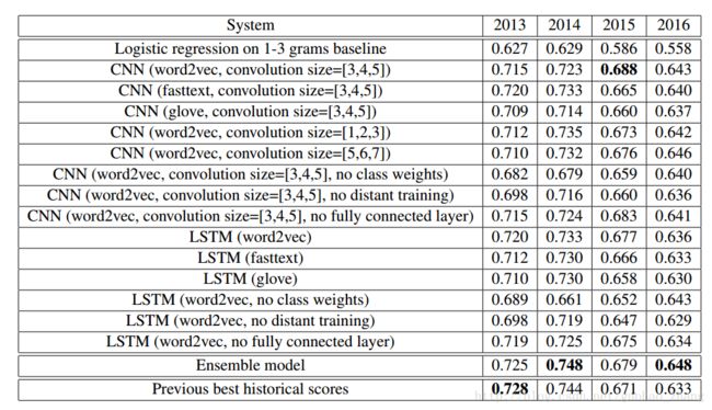
对子任务A的历史测试集的验证结果。粗体值表示给定测试集的最佳分数。
2013年测试集包含3,813条推文，2014年测试集包含1,853条推文，2015年测试集包含2,392条推文，2016年测试集包含20,632条推文。
Word2vec，fasttext和glove指的是无监督阶段的算法选择。
没有类别权重意味着在成本函数中不使用权重来抵消不平衡的类别。
没有distant training意味着我们使用了无监督阶段的嵌入而没有遥远的训练。
没有完全连接的层意味着我们从网络中删除完全连接的隐藏层。
集成模型是指在第二节中描述的集合模型。3.4。
以前最好的历史分数来自（Nakov等，2016）。
他们不是来自一个单一的系统或一个团队; 他们是多年来为每个测试集合获得的最好的分数。

从表1可以看出，GloVe无监督算法比FastText和Word2vec得分低。正是由于这个原因，我们没有在整体模型中包含GloVe变体。

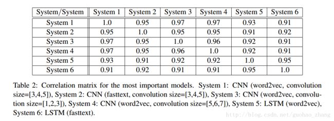
虽然这些individual模型给出了相似的分数，但是他们的输出是足够不相关的，因此将它们相加使分数得到小幅提升。为了弄清楚这些模型是如何相互关联的，我们可以计算任意一对模型的输出概率之间的Pearson相关系数，参见表2.从这张表中我们可以看到，大多数不相关的模型来自不同的监督学习模式（CNN vs. LSTM）和不同的无监督学习

Conclusion

对于未来的工作，探索将CNN和LSTM有机结合起来的系统比通过整体模型更有意思，可能是类似于Stojanovski等人的模型。（2016）。
It would also be interesting to analyze the dependence of the amount of unlabeled and distant data on the performance of the models.
分析未标记数据量和distant数据对模型性能的依赖性也是有意义的。

最后，用阿里云的一个博客 #2017深度学习NLP进展与趋势#
中说到：

3.3.1：SemEval 2017

Twitter中的情感分析不仅引起了NLP研究人员的关注，而且也引起了政治和社会科学界的关注。这就是为什么2013年以来，SemEval大受关注的原因。今年共有48支参赛队参加，为了了解其内容，让我们来看看今年提出的五个子任务：
1. 子任务A：给一则推文，判断其表达的情形：正面，负面或中性。
2. 子任务B：给出一则推文和一个话题，判断主题表达的情感正面与负面。
3. 子任务C：给出一个推文和一个话题，判断推文中传达的情绪等级：强积极，弱积极，中性，弱消极和强消极。
4. 子任务D：给出一组关于话题的推文，判断这组推文在积极和消极之间的分布。
5. 子任务E：给出一组关于某个话题的推文，估计推文在强积极、弱积极、中性、弱消极和强消极的分布情况。
子任务A是最常见的任务，有38个团队参与了这个任务，但是其他的则更具挑战性。主办方表示，DL方法的使用正在不断增加，今年有20个团队使用卷积神经网络（CNN）和长期短期记忆（LSTM）等模型。此外，尽管SVM模型仍然非常流行，但一些参与者将它们与神经网络方法或者使用了词嵌入特征相结合。

3.3.2：BB_twtr系统

今年我发现一个纯的DL系统BB_twtr系统（Cliche，2017）在5 个子任务中排名第一。作者将10个CNN和10个双向LSTM结合起来，使用不同的超参数和不同的预训练策略训练。
为了训练这些模型，作者使用了人工标记的推文（子任务A有49,693个），并且构建了一个包含1亿个推文的未标记数据集，通过简单的标记来提取推特数据集中表示积极的积极表情符号，如:-)，反之亦然消极鸣叫。为了对CNN和双向LSTM输入的词嵌入进行预训练，作者使用word2vec，GloVe和fastText在未标记的数据集上构建词嵌入。然后他使用隔离的数据集来添加积极和消极的信息，然后使用人类标记的数据集再次提炼它们。之前的SemEval数据集的实验表明，使用GloVe会降低性能。然后作者将所有模型与软投票策略结合起来。由此产生的模型比2014年和2016年的历史最好的历史成绩更胜一筹。
这项工作表明了将DL模型结合起来，可以在Twitter中的情感分析中超越监督学习的方法。