Qtoctave安装与使用

GNU Octave (v3.2.4) and QTOctave (v0.9.1) Installation Guide for Windows

GNU Octave Download:

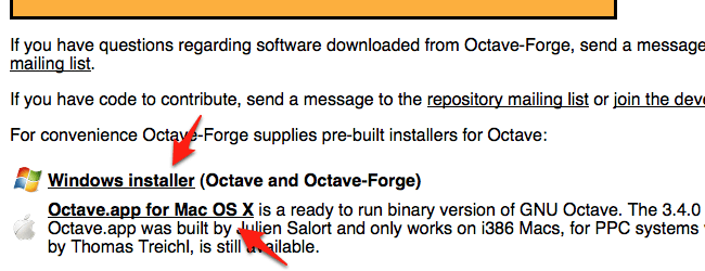
1. Go to http://octave.sourceforge.net/.
2. Click “Windows installer (Octave and Octave-Forge)”.
3. Download and run the executable file.

GNU Octave Installation:

1. Check Octave Forge components. (Leave FFTW3 and ATLAS Libraries with default settings.)
2. Keep default for destination folder.
3. Click Install.

QTOctave Installation:
* Note: Octave must be installed for QTOctave to work

1. Go to http://qtoctave.wordpress.com/download/
2. Click the link under  ">> Windows:" to go to the latest build
3. Download the available qtocatve zip file. (Open with Windows Explorer)
4. Choose "Extract all files" in the window that appears.
5. (Recommended but optional) CHANGE destination folder to C:\Octave\
6. Once extracted, open destination folder qtoctave\bin\
7. Right-click qtoctave.exe and choose "Send to -> Desktop (create shortcut)"
8. Launch QTOctave.

QTOctave Configuration:
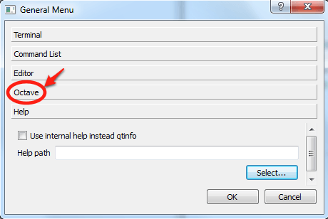
You will receive a warning at launch about selecting the Octave executable:

1. In the Config menu, choose General Configuration, then click Octave.
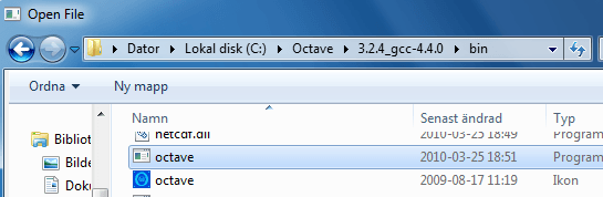
2. Browse to or enter the Octave Path: C:\Octave\3.2.4_gcc-4.4.0\bin\octave.exe
   (When browsing to select the file you may see two files named octave in this directory. Do not select the one with the blue octave application image; it is just an icon file. The other is the executable)
3. Quit and Restart QTOctave to apply changes.

QTOctave died sometime in the year 2011, see https://www.ohloh.net/p/qtoctave.
Personally, I haven't used Octave in a number of years.
Hence: this page is outdated!

Download QtOctave

There are a number of Open Source alternatives to the program MatLab, one of the most known alternatives is GNU Octave. When using Octave you use a command line to enter commands. For a novice, the lack of a graphical interface might be intimidating; QtOctave provides a somewhat user friendly graphical interface to Octave.

Web Interface to Octave

There is a cloud-version of Octave at http://www.verbosus.com/; from this place you can run Octave from the Internet.

Using Ubuntu

Install QtOctave from Ubuntu Software Center.

Octave for Windows or Mac

QtOctave is just a graphical user interface for Octave. In order to run QtOctave, you must first downloadOctave, which can be downloaded from SourceForgehttp://octave.sourceforge.net/. Download it and install it.

Using Mac

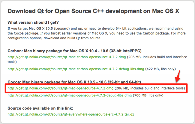
First you need Qt which is a cross-platform C++ application framework. Download Qt fromhttp://qt.nokia.com/downloads/qt-for-open-source-cpp-development-on-mac-os-x/; the file neededis encircled in the picture below, it is the "Cocoa"-file.

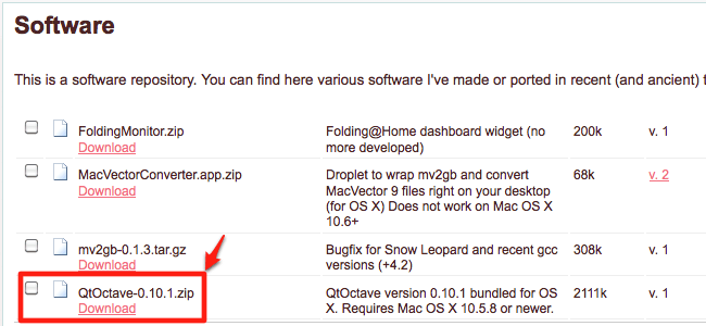
You also need the QtOctave-file which can be downloaded from http://sites.google.com/site/davidecittaro/software.

Double click on the zip-file to extract it, then move the QtOctave-file to the Application folder.

Using Windows

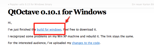
Download QtOctave from http://www.outsch.org/2011/01/29/qtoctave-0-10-1-for-windows/.

Download the zip-file from the link above. Right-click on the zip-file and chooseExtract all. Pick a place where you want the qtoctave-directory. After extracting all files, go to the directory and then into qtoctave/bin, find the file qtoctave.exe, this is the executable file, don't move this file.

You can make a short-cut to the desk top by right-clicking on qtoctave.exe.

When you start QtOctave for the first time you might get an error message saying that it cannot find Octave; the program will start anyway but you will not be able to do anything without Octave. Find the file Octave.exe on your computer, the file is in a directory called bin (binary). Right click on the file and choose properties to see the file path. It might look like this:

C:\Octave\3.2.4_gcc-4.4.0\bin

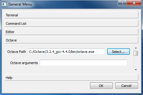
You must now specify this file path in QtOctave. Choose Config->General configuration and click on Octave.

Click on Select... and navigate to the executable Octave-file.

You can also write the file path.

Note that Windows uses "\" to separate directories whereas Unix/Linux uses "/"!

Getting help

If you need help, Google on either MatLab or Octave plus whatever you command/feature you want to know more about. Most of the homepages are made for viewers having a mathematical knowledge exceeding that of a student at school. MatLab is an abbreviation of Matrix Laboratory and the program itself is based on matrices; you can however use the program even though you lack a deeper understanding of linear algebra, in many cases you can think of the matrices simply as tables of numbers.

The Window

The picture below shows the window when starting QtOctave.

There are five tools shown: Variable list, Command List, Navigator, Terminal and Editor. To begin with, you will only need the terminal. The terminal is used when writing commands on one line. If you want to write commands on several lines, you do it using the editor-tool. The commands written in the editor are then saved in so called M-files.

Hide and show tools

You hide a tool by clicking on the small cross at the top of its window.

You show a tool by clicking on the corresponding icon in the tool bar.

You maximize a tool, it will fill up the window, by clicking on the maximize icon or by double clicking atthe menu bar of the tool.

You restore the size by right clicking at the menu bar of the tool and choosingRestore.

As a Calculator

The easiest way to get started, is to use Octave as a calculator.

At the bottom of the terminal there is a command prompt >> followed by an input bar, this is where you enter the commands. After entering a command you press enter and the output will appear above the input bar. You can view the commands you have written in the Command List.

The arithmetic operators are:

+ - * / ^(to the power of)

There are predefined constants in Octave, some of them are listed below:

• pi , e , i
• Inf (infinity)
   
• NaN (not a number)
   

• Make a wild guess!
• Operations yielding numbers larger than the maximum
  floating point will give this answer
• Operations that can not be defined in any reasonably
  way will give this answer

There are also a number of predefined mathematical functions in Octave, some of them are listed below:

• sin, cos, tan
• asin, acos, atan
• exp, log, log10
   
• sqrt
• abs
• round, floor, ceil
• rem

• Trigonometric functions in radians
• Inverse trigonometric functions
• Exponential function, natural logarithm, logarithm to
  the base 10
• Square root
• Absolute value
• Round to nearest integer, round down, round up
• Remainder when doing integer division

Showing more decimals

You can show more decimals by typing format long. Go back to showing few decimals by typingformat short.

---

Exercise 1

Calculate following expressions

Exercise 2

Guess the output of following commands, then check the answers given by Octave

1. 1/0 0/0 tan(pi/2)
2. inf+inf inf-inf inf/inf inf*inf
3. nan+2 nan+nan

Numerical variables

When evaluating the value of an expression, the result is stored in a variable calledans (answer). You can also introduce variables of your own.

Naming variables

Various programs have different rules for naming entities. Although some modern programs allow for all kind of characters in names, you may run into trouble if you use characters like "-" or blank. If you want to stay on the safe side, never having to bother about naming-rules for specific programs, follow these old-school rules:

• The first character must be an english letter : a -z,A - Z
  Some programs can handle letters like å, Æ, Ç, ü; others cannot. Use english names when programming!
• The name can include numbers : 0 - 9
• The name can include underscore : _

These rules apply to Octave and a number of other programs.

Assignments

When writing a=5 at the command prompt, the equal-sign should not be thought of as a logical equality;a is not equal to 5, it is assigned the value 5. Having that in mind, one can write assignments like this

a=a+1

The statement above would be false if it was a logical statement, it is however not a logical statement but an assignment. Theright-hand-side of the statement is calculated first, the result is then assigned to the variable on the left-hand-side.

Hiding the output and repeating previous commands

The recording below shows how to

• Write several commands at one row
• Hide the output by typing semicolon at the end of a command
• Repeat previous commands by using arrows
• Show a list of all variables by showing the Variable List
• Calculate a geometric series

---

Exercise

Calculate the series

The answer is 1.5962

Exercises on Sequences

A sequence is a function with the domain being the natural numbers .

A sequence can be written like this a₀, a₂, a₂,... or like this

Recurrence equations

A geometric progression can be defined in different ways. Consider the infinite geometric progression

You can describe the geometric progression in two ways.

A recurrence equation

An explicit formula

Exercises

Use QtOctave to find the limit as of following sequences. Typeformat long to show more decimals. Try different initial values c, do you get different limits?

Try to explain your answers. If you fail, do the exercises on fixpoints.

Commands and Strings

There is a complete documentation of Octave at http://www.gnu.org/software/octave/doc/interpreter/

Formatting numbers

You can format numbers in three different ways; format long, format short and format bank (2 decimals)

>>> format long
>>> pi
ans = 3.14159265358979
>>> format short
>>> pi
ans = 3.1416
>>> format bank
>>> pi
ans = 3.14 

Just writing the command format will give you the default format short.

String variables

When handling text instead of numbers you use strings. A string is enclosed in either "-signs or '-signs.

>>> my_string_variable="Hello World!"
my_string_variable = Hello World!
>>> my_string_variable='Hello World!'
my_string_variable = Hello World! 

The help command

If you want to find information about a command or a function you can use the help command.

>>> help asin
`asin' is a built-in function

-- Mapping Function: asin (X)

Compute the inverse sine in radians for each element of X.

See also: sin, asind

The disp command

You can use the disp command together with an argument enclosed in brackets to display data. When usingdisp the output is displayed without the ans=.

>>> disp(pi)
3.1416
>>> disp(my_string_variable)
Hello World!
>>> disp("The value of pi is:"), disp(pi)
The value of pi is:
3.1416 

Date and time

When measuring time on a computer it is a convention to measure the time since 00:00:00UTC 1 January 1970. The command time will give you the number of seconds since then; the commandnow will give you the number of days. The command date will give you the current date as a string. The commandclock will give you the current year-month-day-hour-minute-second as a row-matrix.

>>> time
ans = 1.2737e+009
>>> now
ans = 7.3427e+005
>>> date
ans = 12-May-2010
>>> clock
ans =

2010.0000 5.0000 12.0000 15.0000 41.0000 40.3795

m-files

You can store a number of commands in a so called m-file. You enter the commands in the Editor, pickView->Dock Tools->Editor or use the icon at the tool-bar.

The recording below shows how to

• Use the disp command
• Making and using string variables
• Make, save and run a m-file
• Run a m-file from the terminal window

It looks slightly different on the portable version of QtOctave.

视频地址：http://www.malinc.se/math/octave/mfilesen.php

The for-statement

Repeating the same operation over and over again is called iterating. One way to iterate when programming is to use afor statement. A for statement in its simplest form uses a variable representing an index that is increased by 1 in each step.

In the picture to the right the the index is called i. The command betweenfor and end is repeated 10 times. The first time row 2 is executed,i is equal to 0, the second time i is equal to 1, and so on.

Row 4 starts with a %-sign, everything to the right of the %-sign is ignored when the program is run; this is a comment intended for those reading the actual code.

You can increment your index with something else than 1 by adding a number between the starting index and the last index.

1 for i=0:0.1:2
2     disp(i)
3 end
4 %21 numbers are displayed, the numbers 0,0.1,0.2,...,2

The recording below shows various features of the for statement.

视频地址：http://www.malinc.se/math/octave/forstatementen.php

Sequences, Continued

Exercises

Write for-statements in m-files to solve following exercises. Useformat long.

1. The recurrence equation
   
   
   has two fixpoints and .
   Write a for-statement to iterate the recurrence equation 10 times.
   What happens if you start with and respectively?
   What happens if you iterate 50 times? 100 times?
2. Write a recurrence equation for the continued fraction
   
   Hint: it is easier to write a recurrence equation for the continued fraction plus 1.
   
   1. Find the limit of the recurrence equation by iterating in Octave.
   2. Find the exact value of the continued fraction by first finding the fixpoints of the recurrence equation you used in a and then subtracting 1.

further info:

Continued fractions

Some series

A series is said to converge if has a finite limit as.

Exercises

1. Use Octave to make a conjecture about the convergence of
   
   
   as .
2. Use Octave to make a conjecture about the convergence of
   
   
   as .
3. 1. Rewrite the series
      
      using a Σ
   2. Use Octave to make a conjecture about the convergence of this series as
4. Iterate to find the sum of the first 50 terms of
   
   
   then multiply the result with 4. What happens when you iterate 500 times? 5000 times? 50000 times?

further info:

Harmonic series
Madhava-Leibniz series

Comparison Operators

When doing a comparison in Octave you apply a comparison operator on two numbers and the result is eithertrue or false, represented by 1 or 0.

operation

arithmetic operations

logical operations

comparisons

operators

+ - * / ^

&& || !

> >= < <= == !=

operands

numbers

logical values

numbers

result

a number

a logical value

a logical value

The comparison operators are:

>

>=

<

<=

==

!=

greater than, >

greater than or equal to, ≥

less than, <

less than or equal to, ≤

equal to, =

not equal to, ≠

>>> a=1; b=2; c=2; d=3;
>>> a>=b
ans = 0
>>> b>=c
ans = 1
>>> (a < b) && (c!=d)
ans = 1

>>> a < b && c!=d
>>>parse error:

syntax error

>>> a < b && c!=d
^

Boolean Algebra

In Boolean algebra you represent the logical values true and false by the numbers 1 and 0 respectively.

>>> true
ans = 1
>>> false
ans = 0

and, or, not

The basic operators in logic are and, or andnot, these are written using the symbols ∧, ∨ and ¬ respectively. Ifp and q are statements that are either true or false, then you get the truth table

• p
• true
• true
• false
• false

• q
• true
• false
• true
• false

• p ∧ q
• true
• false
• false
• false

• p ∨ q
• true
• true
• true
• false

• ¬p
• false
• false
• true
• true

The operators ∧ and ∨ are binary operators, they are applied to two operands. The operator ¬ is anunary operator, it applies to one operand.

In Octave (and most other programming languages) the operators ∧, ∨ and ¬ are written using the symbols&&, || and !; giving the truth table

• p
• 1
• 1
• 0
• 0

• q
• 1
• 0
• 1
• 0

• p && q
• 1
• 0
• 0
• 0

• p || q
• 1
• 1
• 1
• 0

• !p
• 0
• 0
• 1
• 1

In Octave (and most other programming languages) all numbers that are not 0 are thought of as beingtrue.

>>> a=4.5;
>>> b=0;
>>> (a && b) || !b
ans = 1

Note that you can perform logical operations by using arithmetics.

p && q = pq

p || q = p+q-pq

!p = 1-p

further info:

Fuzzy Logics: This article was published in Scientific American 1993, A Partly True Story, by Ian Stewart

That is true →      ← That is false

Rows and Columns

You create a row matrix consisting of the numbers 4 5 6 7 by entering the numbers inside []-brackets and separating the numbers by a comma or a blank.

>>> r1=[4, 5, 6, 7]

r1 =

4 5 6 7

>>> r2=[4 5 6 7]

r2 =

4 5 6 7

You create a column matrix consisting of the numbers 0.1 0.2 0.3 by entering the numbers inside []-brackets and separating the numbers by a semicolon.

>>> c1=[0.1; 0.2; 0.3]

c1 =

0.10000
0.20000
0.30000

>>> c2=[0.4; 0.5]

c2 =

0.40000
0.50000

Row and column matrices are sometimes called vectors.

You can combine row matrices or column matrices

>>> r=[r1, r2]

r =

4 5 6 4 5 6

>>> c=[c1; c2]

c =

0.10000
0.20000
0.30000
0.40000
0.50000

>>> try_a_mix=[r1, c1]

>>>error: number of rows must match (3 != 1) near line 43, column 16

The first number in a vector has index 1. You can get the number at a specified index.

>>> r(2)
ans = 5
>>> c(5)
ans = 0.50000
>>> r(7)
error: A(I): Index exceeds matrix dimension.

You can use the same notation that creates numbers in for-statements for creating vectors.

>>> r3=3:7
r3 =

3 4 5 6 7

>>> r4=1:3:10
r4 =

1 4 7 10

You can use the same notation for extracting a vector from a vector.

>>> format bank;
>>> r5=0.1:0.1:1
r5 =

0.10 0.20 0.30 0.40 0.50 0.60 0.70 0.80 0.90 1.00

>>> subvector1=r5(2:4)
subvector1 =

0.20 0.30 0.40

>>> subvector2=r5(1:2:10)
subvector2 =

0.10 0.30 0.50 0.70 0.90

You can turn a row into a column or the other way around by doing a transpose using the operator '.

>>> r=[1, 2, 3]
r =

1.00 2.00 3.00

>>> c=r'
c =

1.00
2.00
3.00

Vectors and Scalar

A scalar is just a fancy word for a number; it is used to distinguish numbers from vectors or matrices.

Arithmetic with matrices and scalars

You can use the arithmetic operators +, -, * and/ on a matrix and a scalar. The operation is applied to each element of the matrix.

>>> r=[4, 5, 6]
r =

4.00 5.00 6.00

>>> r1=r*6
r1 =

24.00 30.00 36.00

>>> r2=(r1-20)/2
r2 =

2.00 5.00 8.00

>>> c=[0.5; 3.5]
c =

0.50
3.50

>>> c1=c+0.5
c1 =

1.00
4.00

Functions of matrices

You can apply functions on matrices, the function is then applied to each element of the matrix.

>>> c=[4;16]
c =

4.00
16.00

>>> sqrt(c)
ans =

2.00
4.00

Matrices

A general matrix consists of n rows and m columns.

The recording below shows how to

• create a matrix
• do arithmetic operations with a scalar on a matrix
• find the size by using size(matrix)
• get an element specified by matrix(row,column)
• do comparisons on matrices
• use QtOctave's graphical user interface to handle matrices

---

Exercise

Try the commands ones(3), zeros(4), eye(5)!

视频地址：http://www.malinc.se/math/octave/nmmatricesen.php

Element by Element

You can perform element by element operations on two matrices having the same dimension, i.e. having the same number of rows and columns respectively. When performing an element by element operation the result is a new matrix having the same dimension as the two operands.

When doing an element by element addition, the element on place (row, col) in the resulting matrix will be the sum of the two elements at(row, col) in the operand matrices.

The regular arithmetic operators will become element-by-element operators if you place a dot in front of them.

.+ .- .* ./ .^

>>> m1
m1 =

1 2 3
4 5 6

>>> m2
m2 =

0 1 1
2 2 0

>>> m1./m2
ans =

Inf 2.0000 3.0000
2.0000 2.5000 Inf

>>> m1.^m2
ans =

1 2 3
16 25 1

When applying a function on a matrix the function is applied to each element of the matrix

>>> m=[0 pi pi/2;-pi -pi/2 0]
m =

0.00000 3.14159 1.57080
-3.14159 -1.57080 0.00000

>>> sin(m)
ans =

0.00000 0.00000 1.00000
-0.00000 -1.00000 0.00000

Using element by element operations you can combine comparisons and arithmetic.

>>> m=[1 2 3 4 5; 6 7 8 9 10; 11 12 13 14 15]
m =

1 2 3 4 5
6 7 8 9 10
11 12 13 14 15

>>> m1=m>4
m1 =

0 0 0 0 1
1 1 1 1 1
1 1 1 1 1

>>> m2=m1.*m
m2 =

0 0 0 0 5
6 7 8 9 10
11 12 13 14 15

Regular linear algebra

In regular mathematics, matrix addition and subtraction are defined to be element by element operations. Since using the Octave operators without any dot means "regular" usage, there is no difference between+ and .+, or between - and .-. When it comes to multiplication, division and to-the-power-of, there is a difference between "regular" usage and the element-by-element usage; hence do not use these operators without a dot in front of them (unless you actually know linear algebra).

further info:

GNU Octave, 8.3 Arithmetic Operators bydelorie software

2D Plots

When plotting in Octave you plot points having their x-values stored in one vector and they-values in another vector. The two vectors must be the same size.

You can use a x-vector to store the x-values; then you use element by element operations on thex-vector to store the function values in a y-vector. Having two vectors like this, you then use the command

plot(x_vector, y_vector)

 

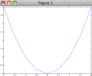
>>> x=-2:2
x =

-2 -1 0 1 2

>>> y=x.^2
y =

4 1 0 1 4

>>> plot(x,y)

Octave inserts lines between the points. If you want a smoother graph, make a longerx-vector.

 

 

>>> x=-2:0.5:2;
>>> y=x.^2;
>>> plot(x,y)

If you know how many points you want to plot in an interval, you can let Octave space the points linearly by using the command

linspace(first x-value, last x-value, number of evenly spaced points)

 

 

>>> x=linspace(-2, 2, 500);
>>> y=x.^2;
>>> plot(x,y)

2D Plots Using GUI

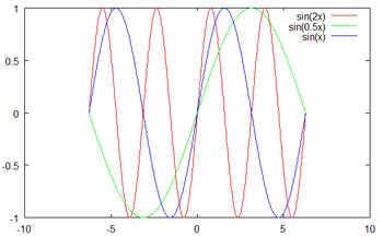
You can use Octave commands to change the appearance of your graphs and to add informative text. If using QtOctave you can use the graphical user interface (GUI) instead of commands.

The recording below shows how to

• use linspace(first value, last value, number of evenly spaced points) to make a vectorx
• make a vector y, where all the elements of y are functions of corresponding elements of the vectorx
• use the command plot(x,y)
• change the appearance of a graph using the QtOctave GUI
• use hold on to draw several graphs in one window (the command hold off turns it off)
• enter labels and titles using the QtOctave GUI
• saving the graph as a png-file using the QtOctave GUI

视频地址：http://www.malinc.se/math/octave/twodusingguien.php

3D the Grid

If we have a function of two variables , we need three axes to display the graph.

When plotting in 2D we use evenly spaced x-values and function values of these stored in ay-vector.

When plotting in 3D we need evenly spaced x- and y-values, spaced on a grid where each function valuez is taken of a point (x, y) on the grid. In order to achieve this we use the command

meshgrid.

>>> x=linspace(-2,2,5)
x =

-2 -1 0 1 2

>>> y=linspace(-2,2,5)
y =

-2 -1 0 1 2

>>> [xx,yy]=meshgrid(x,y)
xx =

-2 -1 0 1 2
-2 -1 0 1 2
-2 -1 0 1 2
-2 -1 0 1 2
-2 -1 0 1 2

yy =

-2 -2 -2 -2 -2
-1 -1 -1 -1 -1
0 0 0 0 0
1 1 1 1 1
2 2 2 2 2

Each point on the grid is made by taken an element from the xx-matrix as thex-value and the corresponding element from the yy-matrix as they-value. All in all there are 25 points in this grid.

3D Plots

After having made a grid you can plot a 3D graph using the command

mesh(xx,yy,z)

where xx and yy are the matrices made by meshgrid and wherez is a function of x and y. You get the function values ofz by using element by element operations on matrices xx andyy.

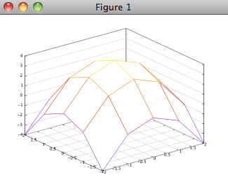
>>> x=linspace(-2,2,5);
>>> y=linspace(-2,2,5);
>>> [xx,yy]=meshgrid(x,y);
>>> mesh(xx,yy,4-(xx.^2+yy.^2))

If you want a smoother graph, make a longer x-vector and a longer y-vector.

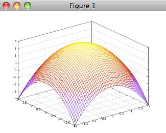
>>> x=linspace(-2,2,50);
>>> y=linspace(-2,2,50);
>>> [xx,yy]=meshgrid(x,y);
>>> mesh(xx,yy,4-(xx.^2+yy.^2))

You can get a contour plot by using the command meshc.

>>> x=linspace(-2,2,50);
>>> y=linspace(-2,2,50);
>>> [xx,yy]=meshgrid(x,y);
>>> meshc(xx,yy,4-(xx.^2+yy.^2))