时间序列--平滑+特征工程

https://machinelearningmastery.com/moving-average-smoothing-for-time-series-forecasting-python/

平滑的希望是消除噪声，更好地揭示潜在的因果过程的信号。移动平均线是时间序列分析和时间序列预测中常用的一种简单的平滑方法。计算移动平均线需要创建一个新的序列，其中的值由原始时间序列中原始观测值的平均值组成。

1.center_ma(t) = mean(obs(t-1), obs(t), obs(t+1))

2.trail_ma(t) = mean(obs(t-2), obs(t-1), obs(t))

计算时间序列的移动平均值需要对数据进行一些假设。假设趋势和季节成分已经从时间序列中移除。这意味着你的时间序列是平稳的，或者没有明显的趋势(长期的增减运动)或者季节性(一致的周期结构)。

例子

原始数据长这样

Date           value
1959-01-01 35
1959-01-02 32
1959-01-03 30
1959-01-04 31
1959-01-05 44

from pandas import Series
from matplotlib import pyplot
series = Series.from_csv('daily-total-female-births.csv', header=0)
# Tail-rolling average transform
rolling = series.rolling(window=3)
rolling_mean = rolling.mean()
print(rolling_mean.head(10))
# plot original and transformed dataset
series.plot()
rolling_mean.plot(color='red')
pyplot.show()

平滑求平均（窗口设为三）之后长这样

Date
1959-01-01          NaN
1959-01-02          NaN
1959-01-03    32.333333
1959-01-04    31.000000
1959-01-05    35.000000
1959-01-06    34.666667
1959-01-07    39.333333
1959-01-08    39.000000
1959-01-09    42.000000
1959-01-10    36.000000

效果图如下

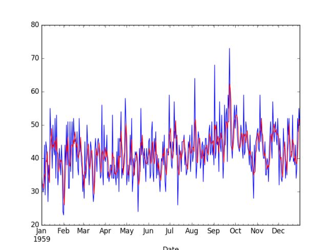
只看前100或许更明显

################现在我把滑动平均当做新特征

之前已有的特征t-1，现在再加一个特征

from pandas import Series
from pandas import DataFrame
from pandas import concat
series = Series.from_csv('daily-total-female-births.csv', header=0)
df = DataFrame(series.values)
width = 3
lag1 = df.shift(1)
lag3 = df.shift(width - 1)
window = lag3.rolling(window=width)
means = window.mean()
dataframe = concat([means, lag1, df], axis=1)
dataframe.columns = ['mean', 't-1', 't+1']
print(dataframe.head(10))

效果如下： 

        mean   t-1     t
0        NaN   NaN   35
1        NaN  35.0   32
2        NaN  32.0   30
3        NaN  30.0   31
4  32.333333  31.0   44
5  31.000000  44.0   29
6  35.000000  29.0   45
7  34.666667  45.0   43
8  39.333333  43.0   38
9  39.000000  38.0   27

这里我们将t-1三个窗口的滑动平均当做新的feature（而不是t时刻的滑动平均）预测t时刻的值

上诉代码的另一种直接实现形式

from pandas import Series
from numpy import mean
from sklearn.metrics import mean_squared_error
from matplotlib import pyplot
series = Series.from_csv('daily-total-female-births.csv', header=0)
# prepare situation
X = series.values
window = 3
history = [X[i] for i in range(window)]
test = [X[i] for i in range(window, len(X))]
predictions = list()
# walk forward over time steps in test
for t in range(len(test)):
	length = len(history)
	yhat = mean([history[i] for i in range(length-window,length)])
	obs = test[t]
	predictions.append(yhat)
	history.append(obs)
	print('predicted=%f, expected=%f' % (yhat, obs))
error = mean_squared_error(test, predictions)
print('Test MSE: %.3f' % error)
# plot
pyplot.plot(test)
pyplot.plot(predictions, color='red')
pyplot.show()
# zoom plot
pyplot.plot(test[0:100])
pyplot.plot(predictions[0:100], color='red')
pyplot.show()

好了，构建新特征之后，我们看一下效果吧

 

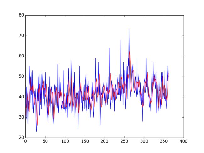
当然不是说这个模型有多好，这只是一个baseline，重点在特征工程的构建上面