浅谈隐式马尔可夫模型 - A Brief Note of Hidden Markov Model (HMM)

Introduction

Problem Formulation

Now we talk about Hidden Markov Model. Well, what is HMM used for? Consider the following problem:

Given an unknown observation: O O , recognize it as one of N N classes with minimum probability of error.

So how to define the error and error probability?
Conditional Error: Given O O , the risk associated with deciding that it is a class i i event:

R(Si|O)=∑j=1NeijP(Sj|O) R ( S i | O ) = ∑ j = 1 N e i j P ( S j | O )

where P(Sj|O) P ( S j | O ) is the probability of that O O is a class Sj S j event and eij e i j is the cost of classifying a class j j event as a class i i event. eij>0,eii=0 e i j > 0 , e i i = 0 .
Expected Error:

E=∫R(S(O)|O)p(O)dO E = ∫ R ( S ( O ) | O ) p ( O ) d O

where S(O) S ( O ) is the decision made on O O based on a policy. Then the question can be considered as:

How should S(O) S ( O ) be made to achieve minimum error probability? Or P(S(O)|O) P ( S ( O ) | O ) is maximized?

Bayes Decision Theory

If we institute the policy: S(O)=Si=argmaxSjP(Sj|O) S ( O ) = S i = arg ⁡ max S j P ( S j | O ) then R(S(O)|O)=minSjR(Sj|O) R ( S ( O ) | O ) = min S j R ( S j | O ) . It is the so-called Maximum A Posteriori (MAP) decision. But how do we know P(Sj|O),i=1,2,…,M P ( S j | O ) , i = 1 , 2 , … , M for any O O ?

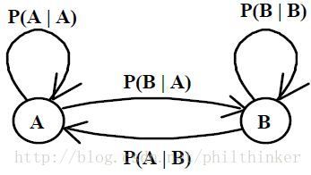
Markov Model

States : S={S0,S1,S2,…,SN} S = { S 0 , S 1 , S 2 , … , S N }
Transition probabilities : P(qt=Si|qt−1=Sj) P ( q t = S i | q t − 1 = S j )
Markov Assumption:

P(qt=Si|qt−1=Sj,qt−1=Sk,…)=P(qt=Si|qt−1=Sj)=aji,aji≥0,∑i=1Naji=1,∀j P ( q t = S i | q t − 1 = S j , q t − 1 = S k , … ) = P ( q t = S i | q t − 1 = S j ) = a j i , a j i ≥ 0 , ∑ i = 1 N a j i = 1 , ∀ j

Hidden Markov Model

States: S={S0,S1,S2,…,SN} S = { S 0 , S 1 , S 2 , … , S N }
Transition probabilities : P(qt=Si|qt−1=Sj)=aji P ( q t = S i | q t − 1 = S j ) = a j i
Output probability distributions (at state j j for symbol k k ): P(yt=Ok|qt=Sj)=bj(k,λj) P ( y t = O k | q t = S j ) = b j ( k , λ j ) parameterized by λj λ j .

HMM Problems and Solutions

1. Evaluation: Given a model, compute probability of observation sequence.
2. Decoding: Find a state sequence which maximizes probability of the observation sequence.
3. Training: Adjust model parameters which maximizes probability of observed sequences.

Evaluation

Compute the probability of observation sequence O=o1o2…oT O = o 1 o 2 … o T , given a HMM model parameter λ λ :

P(O|λ)=∑∀QP(O,Q|λ),Q=q0q1q2…qT=∑∀Qaq0q1bq1(o1)⋅aq1q2bq2(o2)⋯aqT−1qTbqT(oT) P ( O | λ ) = ∑ ∀ Q P ( O , Q | λ ) , Q = q 0 q 1 q 2 … q T = ∑ ∀ Q a q 0 q 1 b q 1 ( o 1 ) ⋅ a q 1 q 2 b q 2 ( o 2 ) ⋯ a q T − 1 q T b q T ( o T )

This is not practical since the number of paths is O(NT) O ( N T ) . How to deal with it?

Forward Algorithm

αt(j)=P(o1o2…ot,qt=Sj|λ) α t ( j ) = P ( o 1 o 2 … o t , q t = S j | λ )

Compute α α recursively:

α0(j)={1,if Sj is the start state0,otherwiseαt(j)=[∑i=0Nαt−1(i)aij]bj(ot),t>0(1)(2) (1) α 0 ( j ) = { 1 , if  S j  is the start state 0 , otherwise (2) α t ( j ) = [ ∑ i = 0 N α t − 1 ( i ) a i j ] b j ( o t ) , t > 0

Then

P(O|λ)=αT(N) P ( O | λ ) = α T ( N )

Computation is O(N2T) O ( N 2 T ) .

Backward Algorithm

βt(i)=P(ot+1ot+2…oT|qt=Si,λ) β t ( i ) = P ( o t + 1 o t + 2 … o T | q t = S i , λ )

Compute β β recursively:

βT(i)={1,if Si is the end state0,otherwiseβt(i)=∑j=0Naijbj(ot+1)βt+1(j),t<T(3)(4) (3) β T ( i ) = { 1 , if  S i  is the end state 0 , otherwise (4) β t ( i ) = ∑ j = 0 N a i j b j ( o t + 1 ) β t + 1 ( j ) , t < T

Then

P(O|λ)=β0(0) P ( O | λ ) = β 0 ( 0 )

Computation is O(N2T) O ( N 2 T ) .

Decoding

Find the state sequence Q Q which maximizes P(O,Q|λ) P ( O , Q | λ ) .

Viterbi Algorithm

VPt(i)=maxq0q1…qt−1P(o1o2…ot,qt=Si|λ) V P t ( i ) = max q 0 q 1 … q t − 1 P ( o 1 o 2 … o t , q t = S i | λ )

Compute VP V P recursively:

VPt(j)=maxi=0,1,…NVPt−1(i)aijbj(ot)t>0 V P t ( j ) = max i = 0 , 1 , … N V P t − 1 ( i ) a i j b j ( o t ) t > 0

Then

P(O,Q|λ)=VPT(N) P ( O , Q | λ ) = V P T ( N )

Save each maximum for backtrace at end.

Training

For the sake of tuning λ λ to maximize P(O|λ) P ( O | λ ) , there is NO efficient algorithm for global optimum, nonetheless, efficient iterative algorithm capable of finding a local optimum exists.

Baum-Welch Reestimation

Define the probability of transiting from Si S i to Sj S j at time t t given O O as1

ξt(i,j)=P(qt=Si,qt+1=Sj|O,λ)=αt(i)aijbj(Ot+1)βt+1(j)P(O|λ) ξ t ( i , j ) = P ( q t = S i , q t + 1 = S j | O , λ ) = α t ( i ) a i j b j ( O t + 1 ) β t + 1 ( j ) P ( O | λ )

Let

a¯ij=Expected num. of trans. from Si to SjExpected num. of trans. from Si=∑T−1t=0ξt(i,j)∑T−1t=0∑Nj=0ξt(i,j)b¯j(k)=Expected num. of times in Sj with symbol kExpected num. of times in Sj=∑t:Ot+1=k∑Ni=0ξt(i,j)∑T−1t=0∑Ni=0ξt(i,j)(5)(6) (5) a ¯ i j = Expected num. of trans. from  S i  to  S j Expected num. of trans. from  S i = ∑ t = 0 T − 1 ξ t ( i , j ) ∑ t = 0 T − 1 ∑ j = 0 N ξ t ( i , j ) (6) b ¯ j ( k ) = Expected num. of times in  S j  with symbol  k Expected num. of times in  S j = ∑ t : O t + 1 = k ∑ i = 0 N ξ t ( i , j ) ∑ t = 0 T − 1 ∑ i = 0 N ξ t ( i , j )

Training Algorithm:

1. Initialize λ=(A,B) λ = ( A , B ) .
2. Compute α,β α , β and ξ ξ .
3. Estimate λ¯=(A¯,B¯) λ ¯ = ( A ¯ , B ¯ ) from ξ ξ .
4. Replace λ λ with λ¯ λ ¯ .
5. If not converge, go to 2.

Reference

More details needed? Refer to :

1. “An Introduction to Hidden Markov Models”, by Rabiner and Juang.
2. “Hidden Markov Models: Continuous Speech Recognition”, by Kai-Fu Lee.

---

• Thanks B. H. Juang in Georgia Institute of Technology.
• Thanks Wayne Ward in Carnegie Mellon University.

---

1. Forward-Backward Algorithm
   ↩