神经网络(以下简称NN)主要用的包是torch.nn。
nn基于autograd,定义模型并微分。一个nn.Module模块包含着forward(input)方法,返回output。
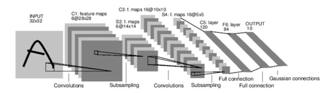
上图是一个简单的前馈网络,从输入一层层向前,算出输出。
典型的训练步骤是:
- 定义NN结构,包括哪些要学习的参数(或权重)
- 迭代计算数据库作为输入
- 将输入传播到整个网络
- 计算损失函数
- 损失反传
- 调整参数,
weight = weight - learning_rate * gradient
定义网络
import torch
from torch.autograd import Variable
import torch.nn as nn
import torch.nn.functional as F
class Net(nn.Module):
    def __init__(self):
        super(Net, self).__init__()
        # 1 input image channel, 6 output channels, 5x5 square convolution
        # kernel
        self.conv1 = nn.Conv2d(1, 6, 5)
        self.conv2 = nn.Conv2d(6, 16, 5)
        # an affine operation: y = Wx + b
        self.fc1 = nn.Linear(16 * 5 * 5, 120)
        self.fc2 = nn.Linear(120, 84)
        self.fc3 = nn.Linear(84, 10)

    def forward(self, x):
        # Max pooling over a (2, 2) window
        x = F.max_pool2d(F.relu(self.conv1(x)), (2, 2))
        # If the size is a square you can only specify a single number
        x = F.max_pool2d(F.relu(self.conv2(x)), 2)
        x = x.view(-1, self.num_flat_features(x))
        # x.view调整大小
        x = F.relu(self.fc1(x))
        x = F.relu(self.fc2(x))
        x = self.fc3(x)
        return x

    def num_flat_features(self, x):
        size = x.size()[1:]  # all dimensions except the batch dimension
        num_features = 1
        for s in size:
            num_features *= s
        return num_features

net = Net()
print(net)
Net (
  (conv1): Conv2d(1, 6, kernel_size=(5, 5), stride=(1, 1))
  (conv2): Conv2d(6, 16, kernel_size=(5, 5), stride=(1, 1))
  (fc1): Linear (400 -> 120)
  (fc2): Linear (120 -> 84)
  (fc3): Linear (84 -> 10)
)
我们定义了前传forward函数,Pytorch会自动求得backward函数,使用autograd可自动计算梯度后传。
可学习的参数可用net.parameters()返回。
params = list(net.parameters())
print(len(params))
print(params[0].size())
10
torch.Size([6, 1, 5, 5])
下面输入一个autograd.Variable变量,输出也是这个类型。
input = Variable(torch.randn(1, 1, 32, 32))
out = net(input)
print out
Variable containing:
 0.0449 -0.0996  0.0021 -0.0830  0.0022 -0.0132 -0.1068  0.1161 -0.0166  0.0630
[torch.FloatTensor of size 1x10]
将梯度缓冲区置零,反传随机梯度:
net.zero_grad()
out.backward(torch.rand(1,10))
注1: 这里手动清零是必须的,因为调用
.backward时Variable.grad会自动累积,即Variable.grad=Variable.grad+new_grad
注2:
torch.nn仅支持一个mini-batch, 整个torch.nn包仅仅支持那些一个mini-batch的输入, 而单独的样本是不行的.
举例,nn.Conv2d须输入一个4维Tensor,形状为nSamples x nChannels x Height x Width.
如果是单独的样本,使用input.unsqueeze(0)去增加batch的伪维度。
我们稍微回顾一下用到的函数和方法。
-
torch.Tensor- 多维度的数组 -
autograd.Variable- *封装一个Tensor,并记录其所有的操作历史。与Tensor有相同的接口,并多一个backward()。 它保留了对tensor的梯度。 -
nn.Module- 神经网络模块。可便捷地整合参数, 并由其他模块辅助进入GPU加速, 输出, 输入, 等等. -
nn.Parameter- 一种自动注册为参数的变量,作为属性分配给模块。 -
autograd.Function-实现前传与后传操作autograd operation的定义。每个变量操作创造至少一个Function节点,链接创造变量的函数,记录操作历史*.
到目前为止,我们 - 定义了一个神经网络
- 处理了输入并调用后传操作
还余下: - 计算损失
- 更新网络权重
损失函数
nn 包里有许多损失函数类型,最简单的是均方差nn.MSEloss。
>>> output = net(input)
>>> target = Variable(torch.range(1, 10))  # a dummy target, for example
__main__:1: UserWarning: torch.range is deprecated in favor of torch.arange and will be removed in 0.3. Note that arange generates values in [start; end), not [start; end].
>>> criterion = nn.MSELoss()
>>> loss = criterion(output, target)
>>> print(loss)
Variable containing:
 37.8372
[torch.FloatTensor of size 1]
>>> output = net(input)
>>> target = Variable(torch.range(1, 10))  # a dummy target, for example
>>> criterion = nn.MSELoss()
>>> loss = criterion(output, target)
>>> print(loss)
Variable containing:
 37.8372
[torch.FloatTensor of size 1]
如果去看loss的.creator属性,会看到计算图就像这样:
input -> conv2d -> relu -> maxpool2d -> conv2d -> relu -> maxpool2d
      -> view -> linear -> relu -> linear -> relu -> linear
      -> MSELoss
      -> loss
当我们调用loss.backward()时,就会调用Loss对整张计算图的导数,变量会计算梯度.grad
print loss.grad_fn
print loss.grad_fn.next_functions[0][0]
print loss.grad_fn.next_functions[0][0].next_functions[0][0]
print loss.grad_fn
print loss.grad_fn.next_functions[0][0]
print loss.grad_fn.next_functions[0][0].next_functions[0][0]
网络反传
调用loss.backward()之前须清理已有的梯度。
net.zero_grad()
print 'conv1.bias.grad before backward'
print net.conv1.bias.grad

loss.backward()

print 'conv1.bias.grad after backward'
print net.conv1.bias.grad
conv1.bias.grad before backward
Variable containing:
 0
 0
 0
 0
 0
 0
[torch.FloatTensor of size 6]

conv1.bias.grad after backward
Variable containing:
1.00000e-02 *
 -2.3452
  8.7239
 -5.3345
 -6.5685
 -2.3857
  5.7952
[torch.FloatTensor of size 6]
更新权重
根据最简单的更新原则随机梯度下降(SGD):
weight = weight - learning_rate * gradient
实现:
lr = 0.01
for f in net.parameters():
  f.data.sub_(f.grad.data * lr)
不过,我们也许希望用更高级的方法,比如Nesterov-SGD,Adam,RMSProp,等等。为了达到这些要求,我们调用torch.optim包:
import torch.optim as optim
optimizer = optim.SGD(net.parameters(), lr=0.01)
optimizer.zero_grad()
output=net(input)
loss = criterion(output, target)
loss.backward()
optimizer.step()