概观

sparklyr为Spark的分布式机器学习库提供绑定。特别是，sparklyr允许访问spark.ml包提供的机器学习例程。与sparklyr的dplyr界面一起，可以轻松地在Spark上创建和调整机器学习工作流程，完全在R中编排。
sparklyr提供了三个功能系列，可以与Spark机器学习一起使用：

用于分析数据的机器学习算法（ml_*）
用于处理各个特征的特征变换器（ft_*）
用于操作Spark DataFrames（sdf_*）的函数

使用sparklyr的分析工作流程可能包含以下几个阶段。有关示例，请参阅示例工作流程。

通过sparklyr dplyr接口执行SQL查询，
使用函数sdf_和ft_函数系列来生成新列或对数据集进行分区，
从ml_*函数族中选择合适的机器学习算法来建模数据，
检查模型拟合的质量，并使用它来预测新数据。
收集结果以便在R中进行可视化和进一步分析

算法

可以通过一ml_*组函数从sparklyr访问Spark的机器学习库：

ml_kmeans K-Means聚类
ml_linear_regression 线性回归
ml_logistic_regression Logistic回归
ml_survival_regression 生存回归
ml_generalized_linear_regression 广义线性回归
ml_decision_tree 决策树
ml_random_forest 随机森林
ml_gradient_boosted_trees 渐变 - 树木
ml_pca 主成分分析
ml_naive_bayes 朴素贝叶斯
ml_multilayer_perceptron 多层感知器
ml_lda 潜在的Dirichlet分配
ml_one_vs_rest 一对阵休息

函数公式

该ml_*函数接受的参数response和features。但features也可以是具有主效应的公式（它目前不接受交互术语）。截取项可以通过使用省略-1。
就是这两种公式展现的方式

ml_linear_regression(z ~ -1 + x + y)
ml_linear_regression(intercept = FALSE, response = "z", features = c("x", "y"))

选项

可以使用ml_options函数中的参数修改Spark模型输出ml_*。这ml_options是专家调整模型输出的唯一界面。例如，model.transform可以在执行拟合之前用于改变Spark模型对象。

转换

Spark提供了特征变换器，促进了Spark DataFrame中数据的许多常见转换，并且Sparklyr在ft_*函数族中公开了这些变换。这些例程通常采用一个或多个输入列，并生成一个新的输出列，形成为这些列的转换。

ft_binarizer 阈值数字特征为二进制（0/1）特征
ft_bucketizer Bucketizer将一列连续特征转换为一列特征桶
ft_discrete_cosine_transform 将时域中的长度NN实值序列变换为频域中的另一长度NN实值序列
ft_elementwise_product 使用逐元素乘法将每个输入向量乘以提供的权重向量。
ft_index_to_string 将一列标签索引映射回包含原始标签作为字符串的列
ft_quantile_discretizer 采用具有连续特征的列，并输出具有分箱分类特征的列
sql_transformer 实现由SQL语句定义的转换
ft_string_indexer 将标签的字符串列编码为标签索引列
ft_vector_assembler 将给定的列列表合并到单个矢量列中

例子

采用数据集iris

library(sparklyr)
library(ggplot2)
library(dplyr)
sc <- spark_connect(master = "local")
iris_tbl <- copy_to(sc, iris, "iris", overwrite = TRUE)
iris_tbt

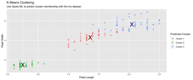
K-MEANS聚类

使用Spark的K-means聚类将数据集分组。K均值聚类将分区指向成k组，使得从点到指定的聚类中心的平方和最小化。

使用k-means聚类

kmeans_model <- iris_tbl %>%
  ml_kmeans(formula = Species~.,centers = 3)

这里需要注意的是，非监督的模型如何写公式

kmeans_model <- iris_tbl %>%
  select(Petal_Width, Petal_Length) %>%
  ml_kmeans(formula = ~.,centers = 3)
kmeans_model
K-means clustering with 3 clusters

Cluster centers:
  Petal_Width Petal_Length
1    1.359259     4.292593
2    0.246000     1.462000
3    2.047826     5.626087

Within Set Sum of Squared Errors =  31.41289

进行预测

predicted <- sdf_predict(kmeans_model, iris_tbl) %>%
  collect

查看聚类的标签和真实的标签之间的关系

table(predicted$Species, predicted$prediction)
         
              0  1  2
  setosa      0 50  0
  versicolor 48  0  2
  virginica   6  0 44

sdf_predict(kmeans_model) %>%
  collect() %>%
  ggplot(aes(Petal_Length, Petal_Width)) +
  geom_point(aes(Petal_Width, Petal_Length, col = factor(prediction + 1)),
             size = 2, alpha = 0.5) + 
  geom_point(data = kmeans_model$centers, aes(Petal_Width, Petal_Length),
             col = scales::muted(c("red", "green", "blue")),
             pch = 'x', size = 12) +
  scale_color_discrete(name = "Predicted Cluster",
                       labels = paste("Cluster", 1:3)) +
  labs(
    x = "Petal Length",
    y = "Petal Width",
    title = "K-Means Clustering",
    subtitle = "Use Spark.ML to predict cluster membership with the iris dataset."
  )

image.png

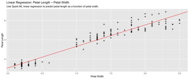
线性回归

建立线性回归模型

lm_model <- iris_tbl %>%
  select(Petal_Width, Petal_Length) %>%
  ml_linear_regression(Petal_Length ~ Petal_Width)

lm_model
Formula: Petal_Length ~ Petal_Width

Coefficients:
(Intercept) Petal_Width 
   1.083558    2.229940 
iris_tbl %>%
  select(Petal_Width, Petal_Length) %>%
  collect %>%
  ggplot(aes(Petal_Length, Petal_Width)) +
  geom_point(aes(Petal_Width, Petal_Length), size = 2, alpha = 0.5) +
  geom_abline(aes(slope = coef(lm_model)[["Petal_Width"]],
                  intercept = coef(lm_model)[["(Intercept)"]]),
              color = "red") +
  labs(
    x = "Petal Width",
    y = "Petal Length",
    title = "Linear Regression: Petal Length ~ Petal Width",
    subtitle = "Use Spark.ML linear regression to predict petal length as a function of petal width."
  )

image.png

逻辑回归

使用Spark的逻辑回归来执行逻辑回归，将二元结果建模为一个或多个解释变量的函数。

数据准备

beaver <- beaver2
beaver$activ <- factor(beaver$activ, labels = c("Non-Active", "Active"))
copy_to(sc, beaver, "beaver")


beaver_tbl <- tbl(sc, "beaver")

建立回归模型

glm_model <- beaver_tbl %>%
  mutate(binary_response = as.numeric(activ == "Active")) %>%
  ml_logistic_regression(binary_response ~ temp)


glm_model <- beaver_tbl %>%
  ml_logistic_regression(activ ~ temp)

> glm_model
Formula: activ ~ temp

Coefficients:
(Intercept)        temp 
  550.52331   -14.69184 

pre <- sdf_predict(glm_model) %>% collect()
pre
# A tibble: 100 x 12
     day  time  temp activ      features  label rawPrediction probability
                              
 1   307   930  36.6 Non-Active   1.00        
 2   307   940  36.7 Non-Active   1.00        
 3   307   950  36.9 Non-Active   1.00        
 4   307  1000  37.2 Non-Active   1.00        
 5   307  1010  37.2 Non-Active   1.00        
 6   307  1020  37.2 Non-Active   1.00        
 7   307  1030  37.2 Non-Active   1.00        
 8   307  1040  36.9 Non-Active   1.00        
 9   307  1050  37.0 Non-Active   1.00        
10   307  1100  36.9 Non-Active   1.00        
# ... with 90 more rows, and 4 more variables: prediction ,
#   predicted_label , probability_0 , probability_1 
>

PCA

使用Spark的主成分分析（PCA）来降低维数。PCA是一种统计方法，用于查找旋转，使得第一个坐标具有可能的最大方差，并且每个后续坐标又具有可能的最大方差
建立PCA模型

pca_model <- tbl(sc, "iris") %>%
  select(-Species) %>%
  ml_pca()


print(pca_model)
Explained variance:

        PC1         PC2         PC3         PC4 
0.924618723 0.053066483 0.017102610 0.005212184 

Rotation:
                     PC1         PC2         PC3        PC4
Sepal_Length -0.36138659 -0.65658877  0.58202985  0.3154872
Sepal_Width   0.08452251 -0.73016143 -0.59791083 -0.3197231
Petal_Length -0.85667061  0.17337266 -0.07623608 -0.4798390
Petal_Width  -0.35828920  0.07548102 -0.54583143  0.7536574

随机森林

使用随机森林进行二分类或者多分类

rf_model <- iris_tbl %>%
  ml_random_forest(Species ~ Petal_Length + Petal_Width, type = "classification",num_trees = 500)



rf_predict <- sdf_predict(rf_model, iris_tbl) %>%
  ft_string_indexer("Species", "Species_idx") %>%
  collect

table(rf_predict$Species_idx, rf_predict$prediction)
     0  1  2
  0 49  1  0
  1  0 50  0
  2  0  0 50

数据集合划分

将Spark DataFrame拆分为训练，测试数据集。

划分数据集合

partitions <- tbl(sc, "iris") %>%
  sdf_partition(training = 0.75, test = 0.25, seed = 1099)

构建线性回归模型

fit <- partitions$training %>%
  ml_linear_regression(Petal_Length ~ Petal_Width)

评价模型的结果

estimate_mse <- function(df){
  sdf_predict(fit, df) %>%
    mutate(resid = Petal_Length - prediction) %>%
    summarize(mse = mean(resid ^ 2)) %>%
    collect
}
sapply(partitions, estimate_mse)

字符串索引

使用ft_string_indexer和ft_index_to_string将字符列转换为数字列，然后再将其转换回来。

ft_string2idx <- iris_tbl %>%
  ft_string_indexer("Species", "Species_idx") %>%
  ft_index_to_string("Species_idx", "Species_remap") %>%
  collect

table(ft_string2idx$Species, ft_string2idx$Species_remap)
        setosa versicolor virginica
  setosa         50          0         0
  versicolor      0         50         0
  virginica       0          0        50

SDF转换

ft_string2idx <- iris_tbl %>%
  sdf_mutate(Species_idx = ft_string_indexer(Species)) %>%
  sdf_mutate(Species_remap = ft_index_to_string(Species_idx)) %>%
  collect

ft_string2idx %>%
  select(Species, Species_idx, Species_remap) %>%
  distinct

简单的例子

让我们通过一个简单的例子来演示在R中使用Spark的机器学习算法。我们将使用ml_linear_regression来拟合线性回归模型。使用内置mtcars数据集，我们将尝试根据车辆的mpg重量（wt）和发动机所包含的气缸数（）来预测汽车的油耗（cyl）。

首先，我们将mtcars数据集复制到Spark中。

mtcars_tbl <- copy_to(sc, mtcars, "mtcars")

使用Spark SQL，功能转换器和DataFrame函数转换数据。

使用Spark SQL删除马力小于100的所有汽车
使用Spark功能变换器将汽车分成两组，基于汽缸
使用Spark DataFrame函数将数据分区为测试和培训
然后使用spark ML拟合线性模型。将MPG作为重量和气缸的函数。

partitions <- mtcars_tbl %>%
  filter(hp >= 100) %>%
  sdf_mutate(cyl8 = ft_bucketizer(cyl, c(0,8,12))) %>%
  sdf_partition(training = 0.5, test = 0.5, seed = 888)



fit <- partitions$training %>%
  ml_linear_regression(mpg ~ wt + cyl)


summary(fit)
 
Deviance Residuals:
    Min      1Q  Median      3Q     Max 
-2.0947 -1.2747 -0.1129  1.0876  2.2185 

Coefficients:
(Intercept)          wt         cyl 
  33.795576   -1.596247   -1.580360 

R-Squared: 0.8267
Root Mean Squared Error: 1.437

这summary()表明我们的模型非常合适，并且汽车重量以及发动机中的汽缸数量都将成为其平均油耗的强大预测因素。（该模型表明，平均而言，较重的汽车消耗的燃料更多。）

让我们使用我们的Spark模型拟合来预测我们的测试数据集的平均油耗，并将预测的响应与真实的测量燃料消耗进行比较。我们将构建一个简单的ggplot2图，使我们能够检查预测的质量。

# Score the data
pred <- sdf_predict(fit, partitions$test) %>%
  collect

# Plot the predicted versus actual mpg
ggplot(pred, aes(x = mpg, y = prediction)) +
  geom_abline(lty = "dashed", col = "red") +
  geom_point() +
  theme(plot.title = element_text(hjust = 0.5)) +
  coord_fixed(ratio = 1) +
  labs(
    x = "Actual Fuel Consumption",
    y = "Predicted Fuel Consumption",
    title = "Predicted vs. Actual Fuel Consumption"
  )

image.png

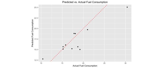
虽然简单，但我们的模型似乎在预测汽车的平均油耗方面做得相当不错。

我们可以轻松有效地将功能变换器，机器学习算法和Spark DataFrame功能组合到Spark和R的完整分析中。

Spark机器学习库（MLlib）

概观

算法

函数公式

选项

转换

例子

K-MEANS聚类

线性回归

逻辑回归

数据准备

PCA

随机森林

数据集合划分

字符串索引

SDF转换

简单的例子

你可能感兴趣的:(Spark机器学习库（MLlib）)