1.Abstract
3.18 3.19 3.20 3.21题
注意:要求作业里面的展示是使用VPython来完成(可以使用动画)
-
EXERCISES
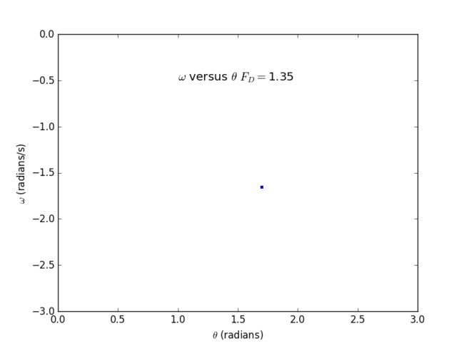
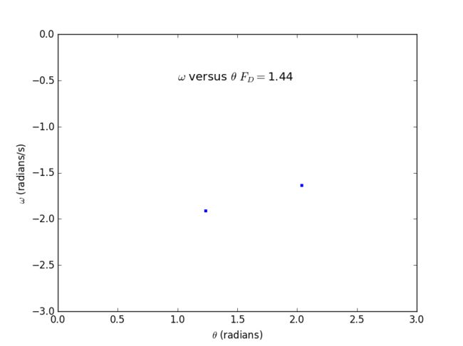
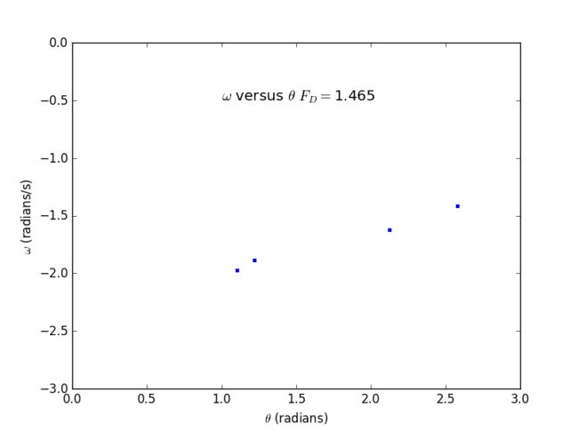
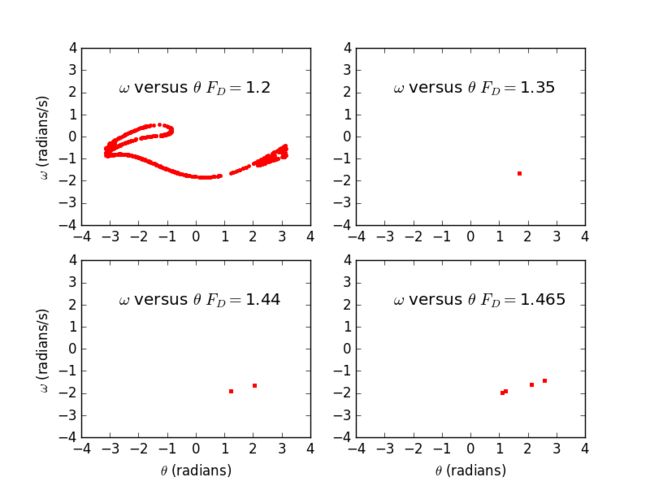
3.18. Calculate Poincaré sections for the pendulum as it undergoes the period-doubling route to chaos. Plot ω versus θ, with one point plotted for each drive cycle, as in Figure 3.9. Do this for FD = 1.4, 1.44, and 1.465, using the other parameters as given in connection with Figure 3.10. You should find that after removing the points corresponding to the initial transient the attractor in the period-1 regime will contain only a single point. Likewise, if the behavior is period n, the attractor will contain n discrete points.
2.Background
-
Poincaré Section (i.e., Poincaré Map)
In mathematics, particularly in dynamical systems, a first recurrence map or Poincaré map, named after Henri Poincaré, is the intersection of a periodic orbit in the state space of a continuous dynamical system with a certain lower-dimensional subspace, called the Poincaré section, transversal to the flow of the system. More precisely, one considers a periodic orbit with initial conditions within a section of the space, which leaves that section afterwards, and observes the point at which this orbit first returns to the section. One then creates a map to send the first point to the second, hence the name first recurrence map. The transversality of the Poincaré section means that periodic orbits starting on the subspace flow through it and not parallel to it.
A Poincaré map can be interpreted as a discrete dynamical system with a state space that is one dimension smaller than the original continuous dynamical system. Because it preserves many properties of periodic and quasiperiodic orbits of the original system and has a lower-dimensional state space, it is often used for analyzing the original system in a simpler way. In practice this is not always possible as there is no general method to construct a Poincaré map.
A Poincaré map differs from a recurrence plot in that space, not time, determines when to plot a point. For instance, the locus of the Moon when the Earth is at perihelion is a recurrence plot; the locus of the Moon when it passes through the plane perpendicular to the Earth's orbit and passing through the Sun and the Earth at perihelion is a Poincaré map. It was used by Michel Hénon to study the motion of stars in a galaxy, because the path of a star projected onto a plane looks like a tangled mess, while the Poincaré map shows the structure more clearly.
-
Logistic Map
The logistic map is a polynomial mapping (equivalently, recurrence relation) of degree 2, often cited as an archetypal example of how complex, chaotic behaviour can arise from very simple non-linear dynamical equations. The map was popularized in a seminal 1976 paper by the biologist Robert May, in part as a discrete-time demographic model analogous to the logistic equation first created by Pierre François Verhulst. Mathematically, don't care about it.
-
Bifurcation Theory
Bifurcation theory is the mathematical study of changes in the qualitative or topological structure of a given family, such as the integral curves of a family of vector fields, and the solutions of a family of differential equations. Most commonly applied to the mathematical study of dynamical systems, a bifurcation occurs when a small smooth change made to the parameter values (the bifurcation parameters) of a system causes a sudden 'qualitative' or topological change in its behaviour. Bifurcations occur in both continuous systems (described by ODEs, DDEs or PDEs) and discrete systems (described by maps). The name "bifurcation" was first introduced by Henri Poincaré in 1885 in the first paper in mathematics showing such a behavior. Henri Poincaré also later named various types of stationary points and classified them.
3.Main
(As usual,In SI, angles in radians)
-
Formulation
In fact, I think there is no necessity to spend extra effort on solving the pendulum problem, because we have already studied it thoroughly from a simple pendulum to pendulum adding dissipation and a driving force. So I will only show the final formula without deriving:
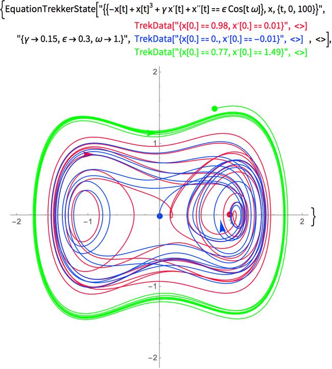
What is new to us is adding the nonlinearity, which transforms the formula into:
Yes, there is nothing new in physics compared with last time.
-
Algorithm
As the authour of our textbook urges, I'd like to use the Euler-Cormer Method to solve this problem (The Pseudocode for subroutine with it is given.)
Yes, there is nothing new in algorithm compared with last time, either.
-
Thinking
In the course of computational physics, when practicing,I will try my best to insist on two princples of programming in my mind:
Simplicity
***As you see, I have dropped the generality for simplicity. ***-
Results
Firstly, I will show all the figures that have emerged in Section 3.1, 3.2, 3.3 to review what I have learned in class.
Secondly, calculate and compare the behavior of two nearly identical pendulums. In detail, calculate the divergence of two nearby tragectories in chaotic regime.
The Figures are as follows:
**☛If you want to enjoy the codes, please click here: code 1 **
**or here: code 2 **
-
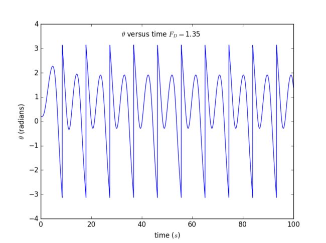
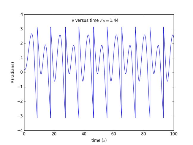
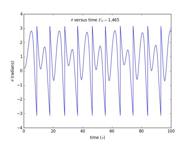
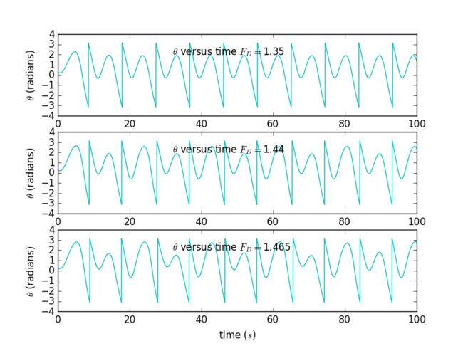
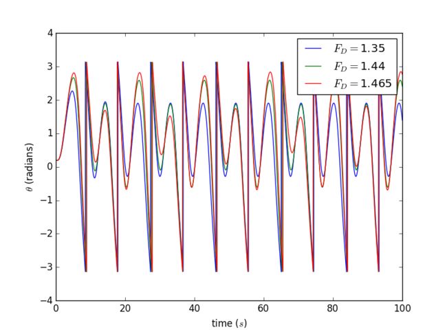
1. Results for θ as a function of time for our pendulum for several different values of the drive amplitude
▶ FD = 1.35
▶ FD = 1.44
▶ FD = 1.465
▶ The first form of combination: subplots
▶ The first form of combination: directly
-
2.Poincaré sections for the pendulum as it undergoes the period-doubling route to chaos
▶ FD = 1.35
▶ FD = 1.44
▶ FD = 1.465
▶ The first form of combination: subplots
4. Conclusion
-
VPython Animation
☛Code: Please click here
-
Qualitative solution:
We have concluded that if the behavior is period n, the attractor will contain n discrete points by plotting.
-
Quantative solution: Not needed
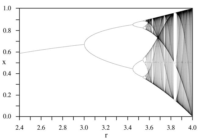
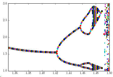
At last, I have collected a beautiful bifurcation diagram for our pendulums.
5. Acknowlegement
- Prof. Cai
- Wikipedia
- Wu Yuqiao
- yuanyuan (Tian Yuan)