姓名:谭善
学号:2014301020106
班级:14级弘毅班
Abstract
A stochastic process (or random process) is a probability model used to describe phenomena that evolve over time or space. It plays quite important role in Statistical and Thermal Physics, especially Thermal Physics. It is so fundamental that it was put in the first chapter in most Thermal textbooks. In this paper, I mainly talked random walks in one, two and three dimension situa-tions. Besides, I disscussed another example about random. Here, I used different functions of python to realize our goals.
1. Backgroud
Stochastic processes were first studied rigorously in the late 19th century to aid in understanding financial markets and Brownian motion. The first person to describe the mathematics behind Brownian motion was Thorvald N. Thiele in a paper on the method of least squares published in 1880. This was followed independently by Louis Bachelier in 1900 in his PhD thesis "The theory of speculation", in which he presented a stochastic analysis of the stock and option markets. Albert Einstein (in one of his 1905 papers) and Marian Smoluchowski (1906) brought the solution of the problem to the attention of physicists, and presented it as a way to indirectly confirm the existence of atoms and molecules. Their equations describing Brownian motion were subsequently verified by the experimental work of Jean Baptiste Perrin in 1908. It boosted the development of physics, so, we are really interested in it.
2. Generation of random number
Random numbers are required in different techniques of statistics, such as when a representative sample is taken from the population as a whole, or when animals are assigned to a different test group or during a Monte Carlo simulation and so on. True random numbers are generated using physical phenomena. But, we can obtain Pseudo random number by using computer.
-
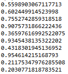
Just like following two groups date. We can get random number using "prob=random.random()" or "x=random.randrange(N)":
This is what we obtained, if you run the program again and again, you will find that there is no regularity about the number we get.
3. Random walks in one dimension
Assuming that a walker that is able to take steps of length unity along a line. And the walker can go left and right, we just want to study its position(or deviation from the origin).
In theory, setting each step as s_i, then, we have
Simplifying it, we have
Now, one can assume that the walker move one step during \Delta t=1, and the walker can go right and left with the same probability. Besides, in order to study the walker's mean position and mean value of x^2. We just looped over 10000 times.
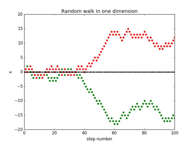
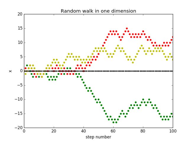
- Following pictures can represent two walkers and three walkers in one dimension, their tracks are random.
Click the Code
From here, we just know that we can predict the walker's track.
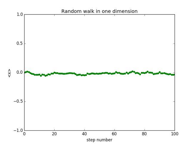
- The following is the figure about the walker's mean displacement.
Click the Code
Obviously, the mean displacement of the walker will fluctuate near 0. In theory, the walker have same probability to go to right and left, so it is not surprising to get this result.
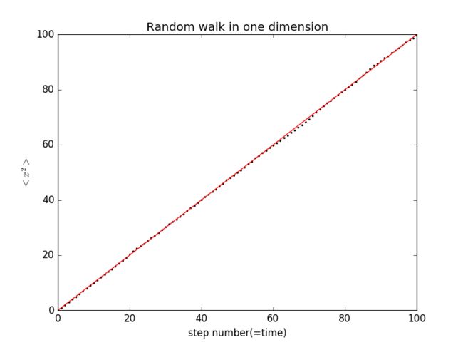
- Instantly, we can plot the mean value of the square of the displacement.
Click the Code
From the figure, we know the mean value of the square of the displacement is in direct proportion to the time t. In theory, we have
So, here, D=1/2
-
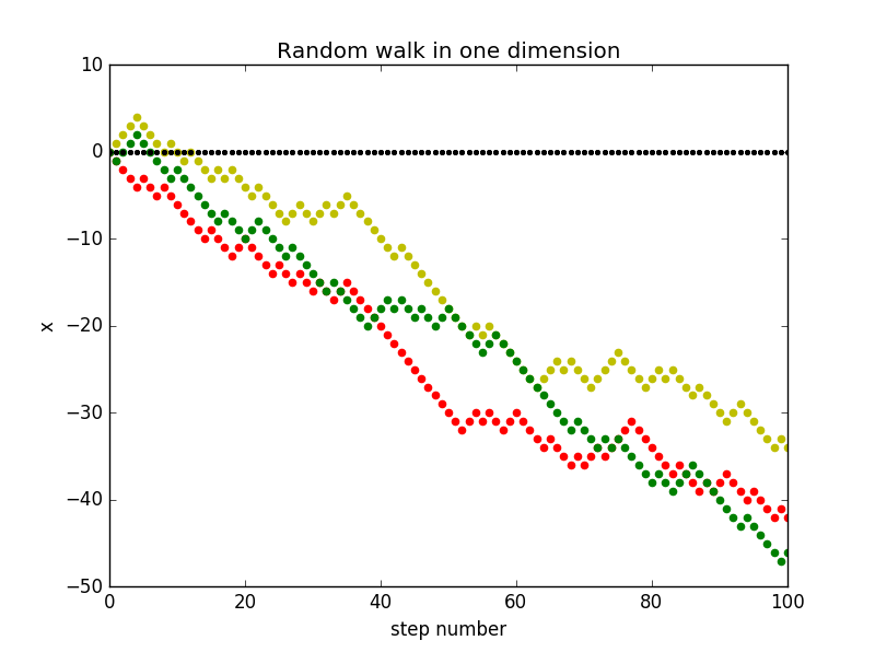
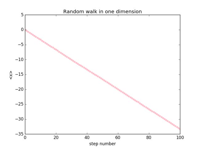
Now, we change the probability about going to left and going to right. Going to right with the probability 1/3 and goint to left with the probability 2/3. We can study some values of this random process. Following two figures represent its track and mean displacement versus time.
-
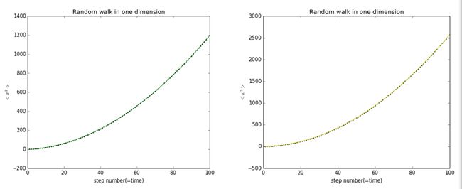
We can change the probability again, and we study the average of the x squared. One situation is that going to right with the probability 1/3 and going to left with the probability 2/3, the other is that going to right with the probability 1/4 and going to left with the probability 3/4.
Although the probability changed, the average of the x squared and time t into a quadratic relationship still. The fits the theory very well.
4. Random walk in two dimension
Python has provided us all kinds of functions, so we can take advantage of them sufficiently. The turtle can help us simulate random walks of two dimension. Assuming that there is a particle in the orign, in the next time-\Delta t, it can go up and down, go left and right with the same probability, then, we can plot its track using random process theory.
- When the length of each step is constant, we have the below picture(left). When the length of each step can be arbitrary range from 0 to 1, we can obtain the following figure(right).
Click the Code
Just like the situation of one dimension, its track is unpredicted. These two figures embodied randomness, it is helpful for us to understand the motion of particles that on the surface.
5. Random walk in three dimension
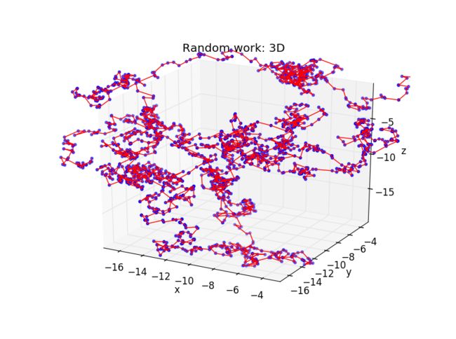
This situation is the most universal situation in our daily life, especially for us who are major in physics. That is because we live in 3-D world. Particles always move in this way. Using python to produce random number, we can simulation particles' motion.
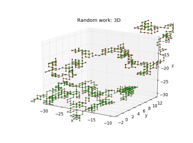
- First, we assume the particle can move in six directions, that is the particle can move along x-axis, y-axis and z-axis. And the particle move one step per time. The length of step is constant. Then, we can obtain these pictures.
Click the Code
Click the Code
Similarily, it given the same results as the situation in one dimension.
-
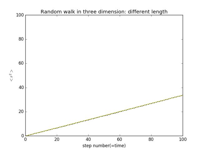
Now, if we consider that each step has different length, the result are given below, the difference is that the relation between the average of the x squared and time t.
-
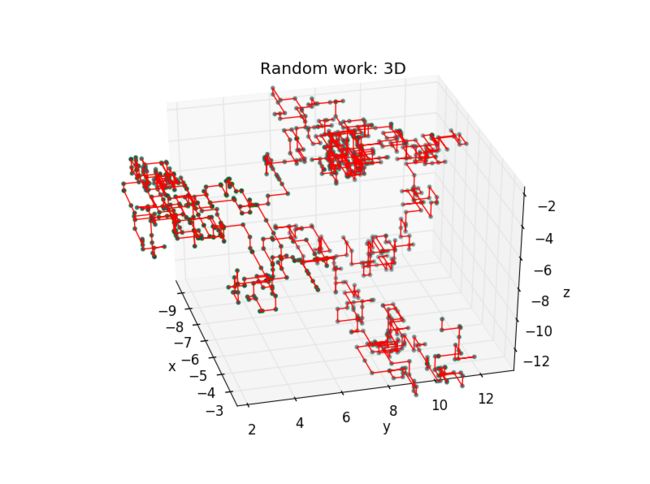
In fact we can find a realer case, that is, the particle can move in all directions, and the length of one step has a range from 0 to 1.
In this case, the motion of particle is more ruleless and random. But in real environment, it is more accuracy. Besides, if we want to use python to get more exact result, we should consider the distribution of mean free path.
6. Random walks and diffusion
consider there is a cup of water, then, we put into a pack of coffee in the center of the water from statistic, we know the density of coffee is then proportional to the probability per unit volume per unit time. From the probability P, we can derive diffusion fuction from random walk.
which leads to
Then
where
If we consider one dimension, we have
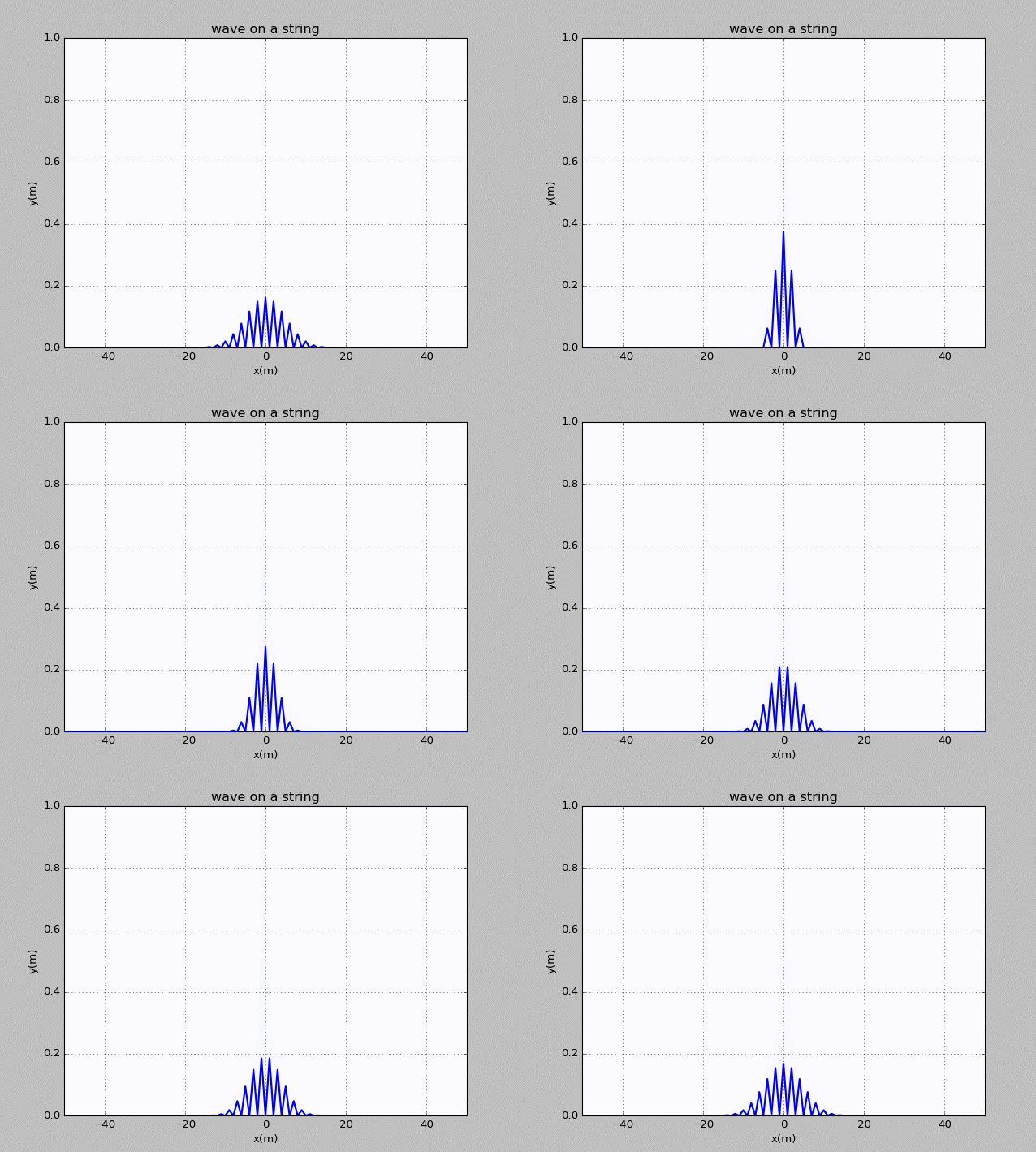
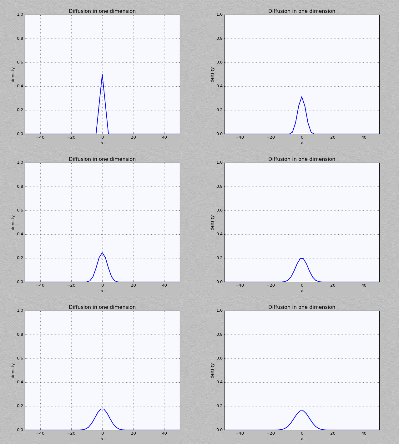
- Consider a particle is at the origin when t=0, then, we study its distribution with time. The following reflected time evolution calculated from the diffusion equation in one dimension.
Click the Code
A curious feature of the results for t>0 is that the density alternates between zero and nonzero values. This behavior is due to the initial density profile which we assumed.
-
We can average the results for adjacent spatial sites so as to "smooth over" the points where the density was zero. Doing this yields the results in the following.
-
I choosed some certain time to plot figures.
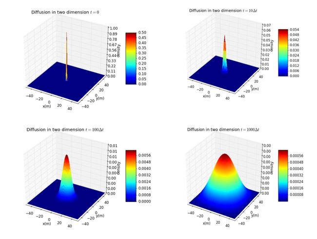
Consider two dimension case, yielding figures below.
Click the Code
In any case, the random-walk results exihibit the Gaussian spreading of the particle distribution.
7. Conclusion
1.For one, two or three dimension, if the particle has same probability move forward to all possible direction, the mean value of the square of the displacement is in direct proportion to the time t.
2. If there are different chances moving to different direction, the average of the x squared and time t into a quadratic relationship.
3. Python provides us all kinds of tools to accomplish our results, we should learn how to apply random number to them.
4. In any case, the random-walk results exihibit the Gaussian spreading of the particle distribution.
8. References
[1] Computational Physics(Second Edition), Nicholas J.Giordano, Hisao Nakanishi.
