本文主要参考文章 http://www.xuebuyuan.com/1248366.html
接收端估计结合文档http://tools.ietf.org/html/draft-alvestrand-rtcweb-congestion-02以及源码webrtc/modules/remote_bitrate_estimator/overuse_detector.cc
添加了一些自己的理解。
webrtc中的带宽自适应算法分为两种:
1、发端带宽控制
原理是由rtcp中的丢包统计来动态的增加或减少带宽,在减少带宽时使用TFRC算法来增加平滑度。
2、收端带宽估算
原理是并由收到rtp数据,估出带宽;用卡尔曼滤波,对每一帧的发送时间和接收时间进行分析,从而得出网络带宽利用情况,修正估出的带宽。
两种算法相辅相成,收端将估算的带宽发送给发端,发端结合收到的带宽以及丢包率,调整发送的带宽。
下面具体分析两种算法:

2 接收端带宽估算算法分析
Each frame is assigned a receive time t(i), which corresponds to the
time at which the whole frame has been received (ignoring any packet
losses). A frame is delayed relative to its predecessor if t(i)-t(i-
1)>T(i)-T(i-1), i.e., if the arrival time difference is larger than
the timestamp difference.
We define the (relative) inter-arrival time, d(i) as
d(i) = t(i)-t(i-1)-(T(i)-T(i-1))
Since the time ts to send a frame of size L over a path with a
capacity of C is roughly
ts = L/C
we can model the inter-arrival time as
d(i) = (L(i)-L(i-1))/C+ w(i) = dL(i)/C+w(i)
带宽估算模型:
d(i) = dL(i) / c + w(i)
其中,d(i)两帧数据的网络传输时间差,dL(i)两帧数据的大小差, c为网络传输能力, w(i)是我们关注的重点, 它主要由三个因素决定:发送速率, 网络路由能力, 以及网络传输能力。w(i)符合高斯分布, 有如下结论:当w(i)增加是,占用过多带宽(over-using);当w(i)减少时,占用较少带宽(under-using);为0时,用到恰好的带宽。所以,只要我们能计算出w(i),即能判断目前的网络使用情况,从而增加或减少发送的速率。
可进一步表示成
d(i) = dL(i) / C(i) + m(i) + v(i)
其中,dL(i)两帧数据的大小差, c为网络传输能力,m(i)为网络抖动(可能大于0:比之前的网络延迟增大;也可以小于0:比之前的网络延迟减小),v(i)为测量误差
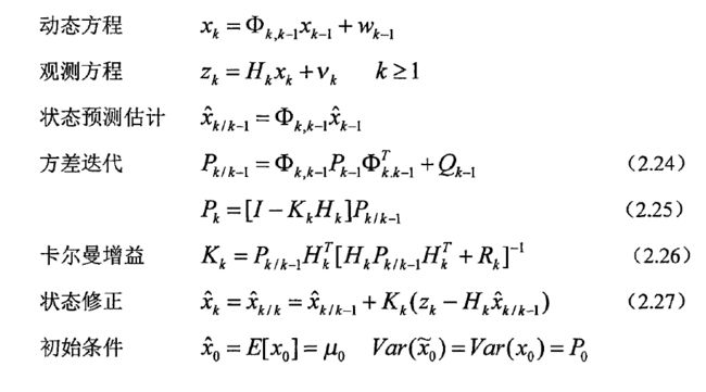
kalman-filters算法原理:
- theta_hat(i) = [1/C_hat(i) m_hat(i)]^T // i时间点的状态由C, m共同表示,theta_hat(i)即此时的估算值
- z(i) = d(i) - h_bar(i)^T * theta_hat(i-1) //d(i)为测试值,可以很容易计算出, 后面的可以认为是d(i-1)对d(i)的估算值, 因此z(i)就是d(i)的偏差,即residual
- theta_hat(i) = theta_hat(i-1) + z(i) * k_bar(i) //好了,这个就是我们要的结果,关键是k值的选取,下面两个公式即是取k值的。最优估计值
- k_bar(i) = (E(i-1) * h_bar(i)) / (var_v_hat + h_bar(i)^T * E(i-1) * h_bar(i))//k_bar(i)为卡尔曼增益,(var_v_hat + h_bar(i)^T * E(i-1) * h_bar(i))即为代码中的denom
- E(i) = (I - K_bar(i) * h_bar(i)^T) * E(i-1) + Q(i) // h_bar(i)由帧的数据包大小算出,E(i)为估计误差协方差阵, Q(i)为过程噪声协方差
由此可见,需要设置初始状态、非测量值的变量有E(0),Q(1),C_hat(0),m_hat(0),
我们只需要知道当前帧的长度,发送时间,接收时间以及前一帧的状态,就可以计算出网络使用情况。
结合卡尔曼滤波的数学公式,可以看出基本匹配。
接下来具体看一下代码
void OveruseDetector::UpdateKalman(int64_t t_delta,
                                   double ts_delta,
                                   uint32_t frame_size,
                                   uint32_t prev_frame_size) {
  const double min_frame_period = UpdateMinFramePeriod(ts_delta);  //最近60帧中,发送间隔最小值
  const double drift = CurrentDrift();
  // Compensate for drift
  const double t_ts_delta = t_delta - ts_delta / drift;  //即d(i)
  double fs_delta = static_cast(frame_size) - prev_frame_size;

  // Update the Kalman filter
  const double scale_factor =  min_frame_period / (1000.0 / 30.0);
  E_[0][0] += process_noise_[0] * scale_factor;  //过程噪声协方差
  E_[1][1] += process_noise_[1] * scale_factor;

  if ((hypothesis_ == kBwOverusing && offset_ < prev_offset_) ||
      (hypothesis_ == kBwUnderusing && offset_ > prev_offset_)) {
    E_[1][1] += 10 * process_noise_[1] * scale_factor;
  }

  const double h[2] = {fs_delta, 1.0}; //即h_bar
  const double Eh[2] = {E_[0][0]*h[0] + E_[0][1]*h[1],
                        E_[1][0]*h[0] + E_[1][1]*h[1]};

  const double residual = t_ts_delta - slope_*h[0] - offset_; //即z(i), slope为1/C

  const bool stable_state =
      (BWE_MIN(num_of_deltas_, 60) * fabsf(offset_) < threshold_);
  // We try to filter out very late frames. For instance periodic key
  // frames doesn't fit the Gaussian model well.
  if (fabsf(residual) < 3 * sqrt(var_noise_)) {
    UpdateNoiseEstimate(residual, min_frame_period, stable_state);
  } else {
    UpdateNoiseEstimate(3 * sqrt(var_noise_), min_frame_period, stable_state);
  }

  const double denom = var_noise_ + h[0]*Eh[0] + h[1]*Eh[1];

  const double K[2] = {Eh[0] / denom,
                       Eh[1] / denom}; //即k_bar

  const double IKh[2][2] = {{1.0 - K[0]*h[0], -K[0]*h[1]},
                            {-K[1]*h[0], 1.0 - K[1]*h[1]}};
  const double e00 = E_[0][0];
  const double e01 = E_[0][1];

  // Update state
  E_[0][0] = e00 * IKh[0][0] + E_[1][0] * IKh[0][1];
  E_[0][1] = e01 * IKh[0][0] + E_[1][1] * IKh[0][1];
  E_[1][0] = e00 * IKh[1][0] + E_[1][0] * IKh[1][1];
  E_[1][1] = e01 * IKh[1][0] + E_[1][1] * IKh[1][1];

  // Covariance matrix, must be positive semi-definite
  assert(E_[0][0] + E_[1][1] >= 0 &&
         E_[0][0] * E_[1][1] - E_[0][1] * E_[1][0] >= 0 &&
         E_[0][0] >= 0);


  slope_ = slope_ + K[0] * residual; //1/C
  prev_offset_ = offset_;
  offset_ = offset_ + K[1] * residual; //theta_hat(i)

  Detect(ts_delta);
}
更新噪声估计
The variance var_v = sigma(v,i)^2 is estimated using an exponential
averaging filter, modified for variable sampling rate
var_v_hat = beta*sigma(v,i-1)^2 + (1-beta)*z(i)^2
beta = (1-alpha)^(30/(1000 * f_max))
where
f_max = max {1/(T(j) - T(j-1))}
for j in i-K+1...i is the highest rate at which frames have been captured by the camera the last K frames and alpha is a filter coefficient typically chosen as a
number in the interval [0.1, 0.001]. Since our assumption that v(i)
should be zero mean WGN is less accurate in some cases, we have
introduced an additional outlier filter around the updates of
var_v_hat. If z(i) > 3 var_v_hat the filter is updated with 3
sqrt(var_v_hat) rather than z(i). For instance v(i) will not be
white in situations where packets are sent at a higher rate than the
channel capacity, in which case they will be queued behind each
other.
结合代码可见,
var_v_hat = beta*sigma(v,i-1)^2 + (1-beta)*z(i)^2
并没有用z(i),而是用avg_noise_ -z(i)。
If z(i) > 3 var_v_hat the filter is updated with 3
sqrt(var_v_hat) rather than z(i)
这句话的实现内容如下:
  if (fabsf(residual) < 3 * sqrt(var_noise_)) {
    UpdateNoiseEstimate(residual, min_frame_period, stable_state);
  } else {
    UpdateNoiseEstimate(3 * sqrt(var_noise_), min_frame_period, stable_state);
  }
可见,webrtc中使用的卡尔曼滤波器是一个自适应的滤波器,即噪声方差自适应变化。
void OveruseEstimator::UpdateNoiseEstimate(double residual,//测量值和预测值之差
                                           double ts_delta,//最小采样间隔
                                           bool stable_state) {
  if (!stable_state) {
    return;
  }
  // Faster filter during startup to faster adapt to the jitter level
  // of the network. |alpha| is tuned for 30 frames per second, but is scaled
  // according to |ts_delta|.
  double alpha = 0.1;// [0.1, 0.001]
  if (num_of_deltas_ > 10*kFrameNumberPerSec) {
    alpha = 0.001;
  }
  // Only update the noise estimate if we're not over-using. |beta| is a
  // function of alpha and the time delta since the previous update.
  const double beta = pow(1 - alpha, ts_delta * kFrameNumberPerSec/ 1000.0);
  avg_noise_ = beta * avg_noise_
              + (1 - beta) * residual;
  var_noise_ = beta * var_noise_
              + (1 - beta) * (avg_noise_ - residual) * (avg_noise_ - residual);
  if (var_noise_ < 1) {
    var_noise_ = 1;
  }
}
过载检测
The offset estimate m(i) is compared with a threshold gamma_1. An
estimate above the threshold is considered as an indication of over-
use. Such an indication is not enough for the detector to signal
over-use to the rate control subsystem. Not until over-use has been
detected for at least gamma_2 milliseconds and at least gamma_3
frames, a definitive over-use will be signaled. However, if the
offset estimate m(i) was decreased in the last update, over-use will
not be signaled even if all the above conditions are met. Similarly,
the opposite state, under-use, is detected when m(i) < -gamma_1. If
neither over-use nor under-use is detected, the detector will be in
the normal state.
评价:思想正确,但是在具体实现要按实际设置gamma_1,gamma_2,gamma_3。
以及其他状态的阀值。
BandwidthUsage OveruseDetector::Detect(double ts_delta) {
 if (num_of_deltas_ < 2) {
   return kBwNormal;
 }
 const double T = BWE_MIN(num_of_deltas_, 60) * offset_; //即gamma_1
 if (fabsf(T) > threshold_) {
   if (offset_ > 0) {
     if (time_over_using_ == -1) {
       // Initialize the timer. Assume that we've been
       // over-using half of the time since the previous
       // sample.
       time_over_using_ = ts_delta / 2;
     } else {
       // Increment timer
       time_over_using_ += ts_delta;
     }
     over_use_counter_++;
     if (time_over_using_ > kOverUsingTimeThreshold  //kOverUsingTimeThreshold是gamma_2, gamama_3=1
         && over_use_counter_ > 1) {
       if (offset_ >= prev_offset_) {
         time_over_using_ = 0;
         over_use_counter_ = 0;
         hypothesis_ = kBwOverusing;
       }
     }
   } else {
     time_over_using_ = -1;
     over_use_counter_ = 0;
hypothesis_ = kBwUnderusing;
   }
 } else {
   time_over_using_ = -1;
   over_use_counter_ = 0;
   hypothesis_ = kBwNormal;
 }
UpdateThreshold(T, now_ms);
return hypothesis_;
}
更新阀值
void OveruseDetector::UpdateThreshold(double modified_offset, int64_t now_ms) {
  if (!in_experiment_)
    return;

  if (last_update_ms_ == -1)
    last_update_ms_ = now_ms;

  if (fabs(modified_offset) > threshold_ + kMaxAdaptOffsetMs) {
    // Avoid adapting the threshold to big latency spikes, caused e.g.,
    // by a sudden capacity drop.
    last_update_ms_ = now_ms;
    return;
  }

  const double k = fabs(modified_offset) < threshold_ ? k_down_ : k_up_;
  const int64_t kMaxTimeDeltaMs = 100;
  int64_t time_delta_ms = std::min(now_ms - last_update_ms_, kMaxTimeDeltaMs);
  threshold_ +=
      k * (fabs(modified_offset) - threshold_) * time_delta_ms;

  const double kMinThreshold = 6;
  const double kMaxThreshold = 600;
  threshold_ = std::min(std::max(threshold_, kMinThreshold), kMaxThreshold);

  last_update_ms_ = now_ms;
}
注意:
threshold_ 和offset之前是一种相互影响的关系。
码率控制
Rate control
The rate control at the receiving side is designed to increase the
receive-side estimate of the available bandwidth A_hat as long as the
detected state is normal. Doing that assures that we, sooner or
later, will reach the available bandwidth of the channel and detect
an over-use.
As soon as over-use has been detected the receive-side estimate of
the available bandwidth is decreased. In this way we get a recursive
and adaptive estimate of the available bandwidth.
In this document we make the assumption that the rate control
subsystem is executed periodically and that this period is constant.
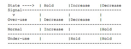
The rate control subsystem has 3 states: Increase, Decrease and Hold.
"Increase" is the state when no congestion is detected; "Decrease" is
the state where congestion is detected, and "Hold" is a state that
waits until built-up queues have drained before going to "increase"
state.
The state transitions (with blank fields meaning "remain in state") are:
参考文档:
http://www.swarthmore.edu/NatSci/echeeve1/Ref/Kalman/ScalarKalman.html
http://tools.ietf.org/html/draft-alvestrand-rtcweb-congestion-02