对于fmri的设计矩阵构造的一个很直观的解释-by 西南大学xulei教授
本程序意在解释这样几个问题:完整版代码在本文的最后。
1.实验的设计如何转换成设计矩阵?


2.设计矩阵的每列表示一个刺激条件,如何确定它们?


3.如何根据设计矩阵和每个体素的信号求得该体素对刺激的敏感性?
程序详解:
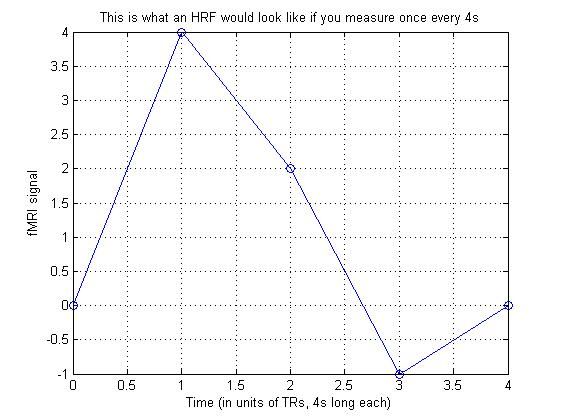
1.构造hrf
hrf_small = [ 0  4  2  -1  0 ];

figure(1);

clf;

plot(0:4,hrf_small,'o-');

grid on;

xlabel('Time (in units of TRs, 4s long each)');

ylabel('fMRI signal');

title('This is what an HRF would look like if you measure once every 4s')
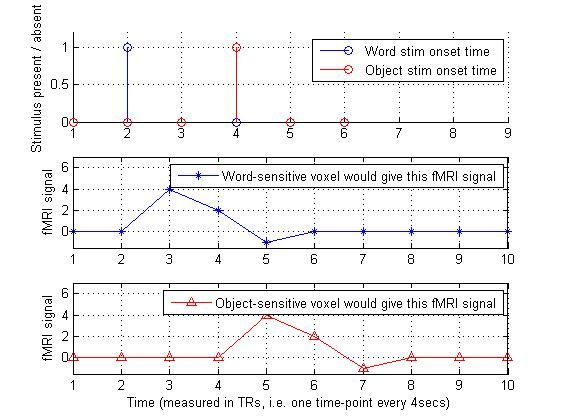
2.构造刺激序列,并与hrf做卷积:
word_stim_time_series =  [ 0 1 0 0 0 0 ];

object_stim_time_series= [ 0 0 0 1 0 0 ];


predicted_signal_that_word_would_evoke = conv(word_stim_time_series,hrf_small);

predicted_signal_that_object_would_evoke = conv(object_stim_time_series,hrf_small);


figure(2);

clf;

subplot(3,1,1);


hold on;


h1=stem(word_stim_time_series,'b');

h2=stem(object_stim_time_series,'r');


hold off;

grid on;

legend([h1(1) h2(1)],'Word stim onset time','Object stim onset time');

axis([1 9 0 1.2]);

ylabel('Stimulus present / absent');

subplot(3,1,2);

plot(predicted_signal_that_word_would_evoke,'b*-');

grid on;

legend('Word-sensitive voxel would give this fMRI signal');

axis([1 10 -1.5 7]);

ylabel('fMRI signal');


subplot(3,1,3);

plot(predicted_signal_that_object_would_evoke,'r^-');


grid on;

legend('Object-sensitive voxel would give this fMRI signal');

axis([1 10 -1.5 7]);

xlabel('Time (measured in TRs, i.e. one time-point every 4secs)');

ylabel('fMRI signal');
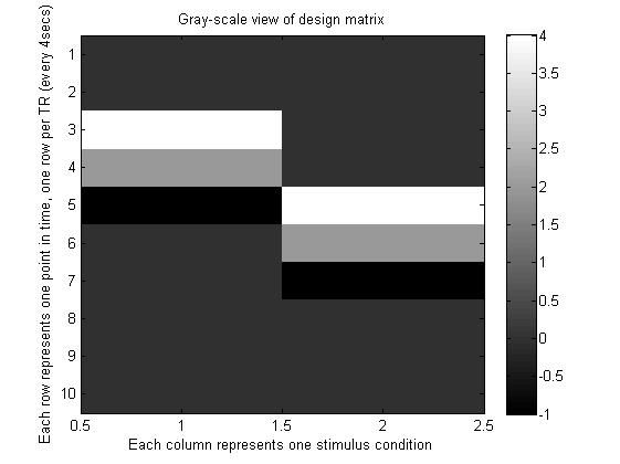
3.利用两个刺激构造设计矩阵,并绘图
predicted_word_response_column_vec = predicted_signal_that_word_would_evoke';


predicted_object_response_column_vec = predicted_signal_that_object_would_evoke';


%%% Now let's look at the actual vectors in the Matlab workspace window


predicted_word_response_column_vec  % Because there is no semi-colon after this,

                                    % it will display in workspace window

predicted_object_response_column_vec


%%%%%% Now we can join these two column vectors together

%%%%%% to make the design matrix. We simply put the two columns side-by-side.

%%%%%% In Matlab, you make new matrices and vectors by

%%%%%% putting the contents inside [ square brackets ]

%%%%%% Note that to join them together in this way, they must be

%%%%%% the same length as each other.

%%%%%%

%%%%%% Because the names of my variables are so long and verbose,

%%%%%% the command below spills over onto two lines. In Matlab,

%%%%%% we can split a command over two lines by putting three dots ...


design_matrix = ...   % The three dots here mean "continued on the next line"

 [ predicted_word_response_column_vec  predicted_object_response_column_vec ];


design_matrix      % No semi-colon, so it displays in window


%%%%%% Translation guide:

%%%%%% In equations, the design matrix is almost always called X

%%%%%% Note that this is a capital "X".

%%%%%%

%%%%%% X = design_matrix;

%%%%%%

%%%%%% Capitals are typically used for matrices, and small-case is

%%%%%% used for vectors.

%%%%%% The only difference between a vector and a matrix is that

%%%%%% a vector is just a bunch of numbers in a row (a row-vector)

%%%%%% or a bunch of numbers in a column (a column-vector),

%%%%%% whereas a matrix is bunch of vectors stacked up next to each

%%%%%% other to make a rectangular grid, with rows *and* columns of numbers.


%%%%%% Now let's view a grayscale plot of the design matrix,

%%%%%% in the way that an fMRI-analysis package, such as SPM, would show it.

%%%%%% To do this, we use the Matlab command "imagesc".

%%%%%% This takes each number in the design matrix and represents

%%%%%% it as a colour, with the colour depending on how big the number is.

%%%%%% In this case, we'll be using a gray colour-scale, so low numbers

%%%%%% will be shown as darker grays, and high numbers are lighter grays.

%%%%%% The "sc" part at the end of "imagesc" stands for "scale", which

%%%%%% means that Matlab scales the mapping of numbers onto colours so

%%%%%% that the lowest number gets shown as black, and the highest as white.

%%%%%%

%%%%%% For examples of how to use the imagesc command to make

%%%%%% pictures of brain-slices, see the companion program

%%%%%% showing_brain_images_tutorial.m


figure(3);

clf;                      % Clear the figure

imagesc(design_matrix);   % 'imagesc' maps the numbers to colors,

                          % normalising so that the max goes to white

                          % and the min goes to black


colormap gray;            % Show everything in gray-scale

colorbar;                 % Shows how the numbers lie on the colour scale

                          % Note that the highest number in the design matrix,

                          % which is 4, is shown as white, and the lowest, -1,

                          % gets shown as black.

title('Gray-scale view of design matrix');

xlabel('Each column represents one stimulus condition');

ylabel('Each row represents one point in time, one row per TR (every 4secs)');
4.设计矩阵和敏感度矩阵相乘,这里假设某一个体素仅仅对某一种刺激有反应,而对另外的刺激没有反应。
%% Now suppose we have a voxel which responds only to words, not to objects.
%% We can calculate how it would be predicted to respond
%% to our word+object display as follows:
%%
%% Predicted response from word-sensitive voxel =
%% 1 * Response which word-presentation would evoke
%% + 0 * Response which object-presentation would evoke
%%
%% Note that this is how the voxel would be predicted to respond
%% if there were no noise whatsoever in the system.
%% Clearly a real fMRI signal would never be this clean.
%%
%% Now, let's make a "sensitivity vector" for this voxel,
%% in which each entry will say how sensitive that voxel is to
%% the corresponding stimulus condition.
%%
%% This voxel is sensitive to words, which are our *first* stimulus-type.
%% And we made the predicted word response into the first column of
%% the design matrix.
%% So, the sensitivity of this voxel to words will be the first element
%% in the sensitivity-vector.
%%
%% Similarly, the sensitivity of this voxel to the second stimulus-type,
%% which are objects, will be the second element in the sensitivity vector.
%%
%% So, the sensitivity vector for a voxel with
%% sensitivity = 1 to the first stimulus-type, which are words
%% and sensitivity = 0 to the second stimulus-type, which are objects
%%
%% will be [ 1 0 ]
%%
%% I know this seems trivial !!
%% Things will get more interesting in a minute...
sensitivity_vec = [ 1 0 ]'; % The dash makes this a column vector
sensitivity_vec % No semi-colon, so it displays in window
%% Translation guide:
%% In equations, the numbers in the sensitivity-vector are typically
%% called "beta-values", or sometimes "beta-coefficients" or "beta-weights".
%% The columns of the design matrix are called "regressors" and
%% the value that is assigned to each regressor is the beta-value.
%%
%% Note that in the example above, we are pretending that we already *know*
%% how sensitive our voxel is to the various stimuli, but in the real world
%% we don't know this. We're trying to figure out what stimuli our voxel
%% is sensitive to, using the fMRI data that we collect in the scanner.
%% This will be described more below.
%% In math-speak, that means that we are trying to *estimate* the betas.
%% When people want to distinguish between the true beta-value
%% (which we don't know) and the estimated beta-value that we figure out
%% from our data, then they call the true one beta and
%% the estimated one "beta hat" (beta with a circumflex sign on top of it: ^
%% [ End of that part of the translation guide, back to the main theme... ]
%% So, we can now express our predicted voxel response in terms
%% of entries in the sensitivity vector multiplied by
%% columns in the design matrix:
%%
%% Predicted response from word-sensitive voxel =
%% 1 * Response which word-presentation would evoke
%% + 0 * Response which object-presentation would evoke
%%
%% And because of the way we made our sensitivity vector and design matrix,
%% this can be re-written as:
%%
%% Predicted response from word-sensitive voxel =
%% (First element in sensitivity vector) * (First column in design matrix)
%% + (Second element in sensitivity vector) * (Second column in design matrix)
%%
%% Here's an important bit:
%% The process above, of going through the elements in a vector,
%% multiplying each element by the corresponding column in a matrix,
%% and then adding up the results of the multiplication,
%% is precisely what matrix multiplication does.
%%
%% In Matlab, everything is by default assumed to be a matrix,
%% (or a vector --- you can think of a vector as simply a matrix that only
%% has one row or column in it), and every multiplication is
%% by default assumed to be a matrix multiplication.
%% So, to matrix-multiply our design matrix by our sensitivity-vector,
%% we just use the standard "multiply by" sign, which is *
predicted_word_selective_voxel_response = design_matrix * sensitivity_vec;
predicted_word_selective_voxel_response
% Let's display this vector in the command window,
% by entering it without a semi-colon after it.
%% When we multiply the design matrix by the sensitivity vector,
%% we make the i-th row of the result by taking the i-th row
%% of the matrix, rotating it 90 degrees, multiplying it element-by-element
%% with the sensitivity vector, and then adding that all up.
%%
%% Since the sensitivity vector is in this case [ 1 0 ],
%% multiplying each matrix row by it element-by-element means that
%% we end up getting 1* the first element in each row, and 0* the second
%% element in each row.
%%
%% So, by the time we have gone through all the rows, we have
%% 1* the first column of the design matrix, plus 0* the second column,
%% which is what we wanted.
%% Let's plot all this
figure(4);
clf; % Clear the figure
subplot(2,1,1); % This is just to make the plots line up prettily
hold on; % "Hold" is one way of putting more than one plot on a figure
h1=plot(predicted_word_response_column_vec,'b*-');
h2=plot(predicted_object_response_column_vec,'r^-');
hold off;
grid on;
legend([h1 h2],'Word-response column vector','Object-response column vector');
axis([1 10 -1.5 7]);
xlabel('Time (measured in TRs, i.e. one time-point every 4secs)');
ylabel('fMRI signal');
subplot(2,1,2);
plot(predicted_word_selective_voxel_response,'ms-'); % Magenta squares
grid on;
legend('Word-selective voxel-response: 1*word-response + 0*object-response');
axis([1 10 -1.5 7]);
xlabel('Time (measured in TRs, i.e. one time-point every 4secs)');
ylabel('fMRI signal');
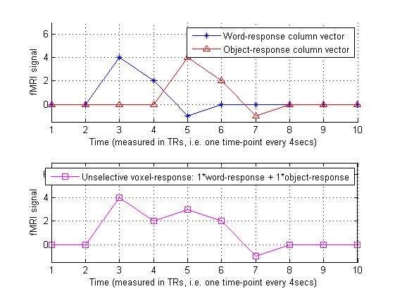
5.假设某一个体素对两种刺激都会产生反应,则它的beta矩阵应当是[1,1]:
%%% Now let's try a voxel which responds equally to both words and objects

%%% So, it's sensitivity vector will be [ 1 1 ]

%%%

%%% This means that its response will be

%%% 1* the first column of the design matrix, plus 1* the second column

%%% i.e.

%%% 1* the response which the word stimulus evokes  +

%%% 1* the response which the object stimulus evokes


sensitivity_vec = [ 1 1 ]';    % The dash makes this a column vector


predicted_unselective_voxel_response = design_matrix * sensitivity_vec;


predicted_unselective_voxel_response     % Display in Matlab command window


%% Let's plot all this


figure(5);

clf;            % Clear the figure

subplot(2,1,1); % This is just to make the plots line up prettily

hold on;        % "Hold" is one way of putting more than one plot on a figure


h1=plot(predicted_word_response_column_vec,'b*-');

h2=plot(predicted_object_response_column_vec,'r^-');


hold off;

grid on;

legend([h1 h2],'Word-response column vector','Object-response column vector');

axis([1 10 -1.5 7]);

xlabel('Time (measured in TRs, i.e. one time-point every 4secs)');

ylabel('fMRI signal');


subplot(2,1,2);

plot(predicted_unselective_voxel_response,'ms-');  % Magenta squares

grid on;

legend('Unselective voxel-response: 1*word-response + 1*object-response');

axis([1 10 -1.5 7]);

xlabel('Time (measured in TRs, i.e. one time-point every 4secs)');

ylabel('fMRI signal');

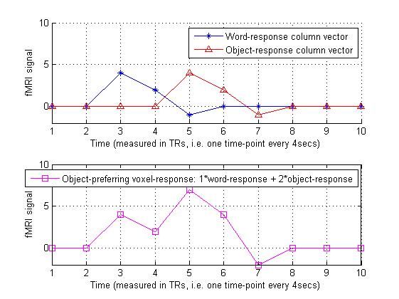
6.假设某一个体素对两种刺激都会产生反应,但是它的beta矩阵是[1,2],即对第二种刺激反应更强烈:
%%% Ok, I hope this isn't overkill: let's try a voxel which gives a normal

%%% response to words, but which gives a response to objects which is

%%% *twice* as strong.

%%% So, it's sensitivity vector will be [ 1 2 ]

%%%

%%% This means that its response will be

%%% 1* the first column of the design matrix, plus 2* the second column

%%% i.e.

%%% 1* the response which the word stimulus evokes  +

%%% 2* the response which the object stimulus evokes


sensitivity_vec = [ 1 2 ]';   % The dash makes this a column vector


predicted_object_preferring_voxel_response = design_matrix * sensitivity_vec;


predicted_object_preferring_voxel_response    % Display in Matlab command window


%% Let's plot all this


figure(6);

clf;            % Clear the figure

subplot(2,1,1); % This is just to make the plots line up prettily

hold on;


h1=plot(predicted_word_response_column_vec,'b*-');

h2=plot(predicted_object_response_column_vec,'r^-');


hold off;

grid on;

legend([h1 h2],'Word-response column vector','Object-response column vector');

axis([1 10 -2 10]);

xlabel('Time (measured in TRs, i.e. one time-point every 4secs)');

ylabel('fMRI signal');


subplot(2,1,2);

plot(predicted_object_preferring_voxel_response,'ms-');  % Magenta squares

grid on;

legend('Object-preferring voxel-response: 1*word-response + 2*object-response');

axis([1 10 -2 10]);

xlabel('Time (measured in TRs, i.e. one time-point every 4secs)');

ylabel('fMRI signal');
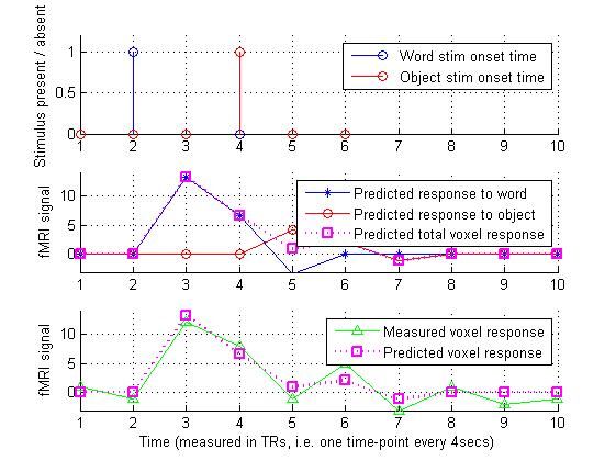
7.我们现在模拟出一个真实测量得到的生理信号体素激活值:
measured_voxel_data = [ 1  -1  12  8  -1  5  -3 1  -2  -1 ]';


% This is is what often gets called "y".

% This measured signal is probably some kind of mixture of

% a response to the word stimulus and a response to the object stimulus,

% with random noise thrown on top.


% Let's plot it


figure(7);

clf;                % Clear the figure

plot(measured_voxel_data,'o-');

                    % Plot HRF against time, with one time-point every TR seconds.

                    % A line with circles on it

grid on;

xlabel('Time (in units of TRs, 4s long each)');

ylabel('fMRI signal');

title('Measured voxel data');

8.进行数据拟合,矩阵求逆,求伪逆,然后绘图plot,进行比对:
%%% What is the estimated sensitivity vector of this voxel ?

%

% Well, we make the pseudo-inverse of the design matrix, and multiply

% it by the vector of measured voxel data:


estimated_voxel_sensitivity = pinv(design_matrix) * measured_voxel_data;


%%% This estimated_voxel_sensitivity is what gets called beta-hat in the math.


%%% Let's display this in the workspace, by typing it without a semi-colon


estimated_voxel_sensitivity


%%% This makes the following show up in the Matlab command window:

%

% estimated_voxel_sensitivity =

%

%    3.2965

%    1.0565

%

%%% So, the estimate is that this voxel is around 3 times more sensitive to

%%% words than it is to objects


%%% Now, let's make a plot of what the predicted response would be of

%%% a voxel that has a sensitivity matrix which is *exactly* our estimate,

%%% and compare it to the voxel response which we measured.

%%% They won't be exactly the same, because of the noise in the signal.


predicted_voxel_output = design_matrix * estimated_voxel_sensitivity;


%%% This predicted overall voxel output is just the

%%% predicted response to the word, plus the predicted response to the object.

%%% As we saw in hrf_tutorial.m, the idea that we can calculate the overall

%%% response simply by adding up these two separate responses is what it

%%% means to say that we are assuming that the system is LINEAR.

%%%

%%% If we want to look at the predicted responses to the separate stimulus

%%% types, we can calculate them by separately multiplying the

%%% corresponding column of the design matrix by the corresponding element

%%% of the estimated sensitivity vector.


predicted_response_to_word = predicted_word_response_column_vec * ...

                             estimated_voxel_sensitivity(1);


predicted_response_to_object = predicted_object_response_column_vec * ...

                               estimated_voxel_sensitivity(2);


%%%%% Let's plot all this


figure(8);

clf;            % Clear the figure


subplot(3,1,1); % This is just to make the plots line up prettily

hold on;


h1=stem(word_stim_time_series,'b');

h2=stem(object_stim_time_series,'r'); % Word onset in blue, object onset in red


hold off;

grid on;

legend([h1(1) h2(1)],'Word stim onset time','Object stim onset time');

axis([1 10 0 1.2]); % This just sets the display graph axis size

ylabel('Stimulus present / absent');


subplot(3,1,2);

hold on;

h1=plot(predicted_response_to_word,'b*-');

h2=plot(predicted_response_to_object,'ro-');

h3=plot(predicted_voxel_output,'ms:','linewidth',2);

                %%% 'ms:' means plot in the colour magenta (m),

                %%% with squares as the markers (s), using a dotted line (:).

                %%% Then we make the width of the line broader, linewidth=2,

                %%% so that it shows up better.

                %%% Note that the predicted_voxel_output is simply the sum of

                %%% predicted_response_to_word and predicted_response_to_object

grid on;

legend([h1 h2 h3],'Predicted response to word', ...

              'Predicted response to object','Predicted total voxel response');


axis([1 10 -3 14]);

ylabel('fMRI signal');


subplot(3,1,3);

hold on;

h1=plot(measured_voxel_data,'g^-');

h2=plot(predicted_voxel_output,'ms:','linewidth',2);

hold off;

grid on;

legend([h1 h2],'Measured voxel response','Predicted voxel response');

axis([1 10 -3 14]);

xlabel('Time (measured in TRs, i.e. one time-point every 4secs)');

ylabel('fMRI signal');
%%%% Tutorial on the basic structure of an fMRI design matrix, using Matlab

%%%% Written by Rajeev Raizada, July 23, 2002.

%%%%

%%%% This file follows up on a preceding one: hrf_tutorial.m

%%%%

%%%% Neither file assumes any prior knowledge of linear algebra

%%%%

%%%% Please mail any comments or suggestions to: raizada at cornell dot edu

%%%%

%%%% Probably the best way to look at this program is to read through it

%%%% line by line, and paste each line into the Matlab command window

%%%% in turn. That way, you can see what effect each individual command has.

%%%%

%%%% Alternatively, you can run the program directly by typing

%%%%

%%%%   design_matrix_tutorial

%%%%

%%%% into your Matlab command window.

%%%% Do not type ".m" at the end

%%%% If you run the program all at once, all the Figure windows

%%%% will get made at once and will be sitting on top of each other.

%%%% You can move them around to see the ones that are hidden beneath.

%%%%

%%%% Note that this tutorial only shows the method where the

%%%% design matrix assumes a specific shape to the HRF.

%%%% It is also possible to estimate the HRF without making

%%%% any assumptions about its shape. This is called using the

%%%% Finite Impulse Response method, or FIR.

%%%% This involves using a slightly more complicated design-matrix

%%%% than the one we make below.

%%%%

%%%% First, let's make a pretend mini-hrf, just to show examples.

%%%% This is similar in shape to the HRFs that we looked at in

%%%% the program hrf_tutorial.m, but it doesn't have as many time-points.

%%%% One reason to use a shortened HRF like this is just to save typing!

%%%% But in fact, this is approximately what a real HRF would look like

%%%% if you only measured from it once every four seconds.

%%%% In fMRI, the time it takes to make a whole-brain measurement is called

%%%% the TR (Time for Repetition, although people say "Repetition Time").

%%%% So, this HRF is similar to what we'd measure

%%%% if our scanner had a TR of 4 seconds. These days, fast scanners

%%%% can usually manage to get a whole-brain full of data in only 2s.


hrf_small = [ 0  4  2  -1  0 ];


%%%% Plot it


figure(1);

clf;                        % Clear the figure

plot(0:4,hrf_small,'o-');   % Plot HRF against a time-vector [0,1,2,3,4]

                            % 'o-' means "use a line with circles on it"

                            % Type "help plot" in the Matlab command window

                            % to get a list of all the line-styles and markers

                            % that you can use. There are lots of them!


grid on;                    % Overlay a dotted-line grid on top of the plot

xlabel('Time (in units of TRs, 4s long each)');

ylabel('fMRI signal');

title('This is what an HRF would look like if you measure once every 4s')


%%%%%%%%%%%%%%%%%%%%%%%%%%%%%%%%%%%%%%%%%%%%%%%%%%%%%%%%%%%%%%%%%%

%

% Just as we did in hrf_tutorial.m, now we're going to make

% a time-series of 1's and 0's representing the times when stimuli

% are shown. These time-series will be convolved with the HRF,

% in order to see what kinds of fMRI signals would be evoked in voxels

% that respond to the stimuli. These predicted responses will form

% the columns of our design matrix, as is shown in more detail below.

%

% Just for purposes of illustration, we're going to imagine that

% one of our stimuli is flashing up a word on the screen, and that

% the other is flashing up a picture of an object.

%

% These stimulus onsets will probably produce more complex patterns

% of neural firing than the sudden flash of light that we talked about

% in HST_hrf_tutorial.m, but we're going to ignore that complication

% for now. We'll simply suppose that each stimulus instantly kicks off

% its own standard-shaped HRF.

% This is what's typically done in event-related fMRI, and it turns

% out that it usually works pretty well.


%%%%%%%%%%%%%%% Now suppose we present a word at time t=2


word_stim_time_series =  [ 0 1 0 0 0 0 ];


%%%%%%%%%%%%%%% And let's present a picture of an object at time t=4


object_stim_time_series= [ 0 0 0 1 0 0 ];


%%%% Let's convolve these with our mini-HRF to see what kind of fMRI

%%%% signals they would evoke in voxels which respond to words or pictures


predicted_signal_that_word_would_evoke = conv(word_stim_time_series,hrf_small);


predicted_signal_that_object_would_evoke = conv(object_stim_time_series,hrf_small);


%%% Let's plot all this


figure(2);

clf;            % Clear the figure

subplot(3,1,1); % This is just to make the plots line up prettily.

                % The first number is how many rows of subplots we have: 3

                % The second number is how many columns: 1

                % The third number is which subplot to draw in: the first one.

                % So, we end up with three plots stacked on top of each other,

                % and we draw in the first one (which is the uppermost subplot)


hold on;        % "Hold" is one way of putting more than one plot on a figure


h1=stem(word_stim_time_series,'b');

                % Stem makes a nice looking plot with lines and circles

h2=stem(object_stim_time_series,'r'); % Word onset in blue, object onset in red

                % The "h1=" and "h2=" bits are called "handles".

                % They are pointers to the plots that we are making,

                % which are the stem plots in this case.

                % Making handles like this is useful for manipulating

                % pretty much any aspect of the plot afterwards.

                % In this instance, we use them to put a legend on the plot.

                % That's done by the "legend" command, a couple of lines below.

                % There's no need to worry about these handles at this stage,

                % I just wanted to explain what those mysterious-looking h's

                % were doing there. Usually you can make a nice-looking legend

                % without worrying about handles, but it turns out that

                % for stem plots they help to make the legend look better.

hold off;

grid on;

legend([h1(1) h2(1)],'Word stim onset time','Object stim onset time');

                % We use the h1 and h2 handles here.

                % This helps us to get the right symbols displayed in the legend,

                % in this case, blue and red circles.


axis([1 9 0 1.2]);  % This just sets the display graph axis size

                    % The first two numbers are the x-axis range: 1 to 9

                    % The last two numbers are the y-axis range: 0 to 1.2

ylabel('Stimulus present / absent');


subplot(3,1,2);

plot(predicted_signal_that_word_would_evoke,'b*-');

                                    % 'b*-' means blue stars on a solid line

grid on;

legend('Word-sensitive voxel would give this fMRI signal');

axis([1 10 -1.5 7]);

ylabel('fMRI signal');


subplot(3,1,3);

plot(predicted_signal_that_object_would_evoke,'r^-');

                                    % 'r^-' means red triangles

                                    % pointing up, lying on a solid line.

grid on;

legend('Object-sensitive voxel would give this fMRI signal');

axis([1 10 -1.5 7]);

xlabel('Time (measured in TRs, i.e. one time-point every 4secs)');

ylabel('fMRI signal');


%%%%%%%%%%%%%%%%%%%%%%%%%%%%%%%%%%%%%%%%%%%%%%%%%%%%%%%%%%%%%%%%%%%%%%

%%%%%%

%%%%%% What the design matrix has in it

%%%%%%

%%%%%%%%%%%%%%%%%%%%%%%%%%%%%%%%%%%%%%%%%%%%%%%%%%%%%%%%%%%%%%%%%%%%%%

%%%%%%

%%%%%% Here's the key part.

%%%%%% The design matrix is built up out of these predicted responses.

%%%%%%

%%%%%% Each column of the design matrix is the predicted fMRI signal

%%%%%% that a voxel would give, if it were perfectly and exclusively

%%%%%% sensitive to a particular stimulus-condition.

%%%%%%

%%%%%% In our case, the first column of the design matrix

%%%%%% would be the vector "predicted_signal_that_word_would_evoke"

%%%%%% that we made just above, and the second column would be

%%%%%% the vector "predicted_signal_that_object_would_evoke"

%%%%%%

%%%%%% So, the most important part of the design matrix

%%%%%% is simply these two vectors side-by-side.

%%%%%%

%%%%%% A real design matrix would have some other columns in it too,

%%%%%% which have other types of predicted fMRI signals in them,

%%%%%% e.g. what the signal would look like if the scanner's output

%%%%%% were slowly drifting in time.

%%%%%% But those other columns don't deal with the signal that the stimuli

%%%%%% would be predicted to evoke in the brain, and so we can ignore them

%%%%%% for now. (Later in the HST583 course, Doug will talk more about

%%%%%% how you might model slow-scanner drift etc.)

%%%%%%

%%%%%% It's the *columns* of the design matrix that get built up out of

%%%%%% these predicted responses to the different stimulus types,

%%%%%% but the actual vectors that we made above are row vectors,

%%%%%% i.e. just a bunch of numbers in a row.

%%%%%% So, to match the format of the design matrix, we need to turn

%%%%%% these into column vectors, by transposing them (i.e. flipping them).

%%%%%% We do this by putting a dash/apostrophe at the end of the vector


predicted_word_response_column_vec = predicted_signal_that_word_would_evoke';


predicted_object_response_column_vec = predicted_signal_that_object_would_evoke';


%%% Now let's look at the actual vectors in the Matlab workspace window


predicted_word_response_column_vec  % Because there is no semi-colon after this,

                                    % it will display in workspace window

predicted_object_response_column_vec


%%%%%% Now we can join these two column vectors together

%%%%%% to make the design matrix. We simply put the two columns side-by-side.

%%%%%% In Matlab, you make new matrices and vectors by

%%%%%% putting the contents inside [ square brackets ]

%%%%%% Note that to join them together in this way, they must be

%%%%%% the same length as each other.

%%%%%%

%%%%%% Because the names of my variables are so long and verbose,

%%%%%% the command below spills over onto two lines. In Matlab,

%%%%%% we can split a command over two lines by putting three dots ...


design_matrix = ...   % The three dots here mean "continued on the next line"

 [ predicted_word_response_column_vec  predicted_object_response_column_vec ];


design_matrix      % No semi-colon, so it displays in window


%%%%%% Translation guide:

%%%%%% In equations, the design matrix is almost always called X

%%%%%% Note that this is a capital "X".

%%%%%%

%%%%%% X = design_matrix;

%%%%%%

%%%%%% Capitals are typically used for matrices, and small-case is

%%%%%% used for vectors.

%%%%%% The only difference between a vector and a matrix is that

%%%%%% a vector is just a bunch of numbers in a row (a row-vector)

%%%%%% or a bunch of numbers in a column (a column-vector),

%%%%%% whereas a matrix is bunch of vectors stacked up next to each

%%%%%% other to make a rectangular grid, with rows *and* columns of numbers.


%%%%%% Now let's view a grayscale plot of the design matrix,

%%%%%% in the way that an fMRI-analysis package, such as SPM, would show it.

%%%%%% To do this, we use the Matlab command "imagesc".

%%%%%% This takes each number in the design matrix and represents

%%%%%% it as a colour, with the colour depending on how big the number is.

%%%%%% In this case, we'll be using a gray colour-scale, so low numbers

%%%%%% will be shown as darker grays, and high numbers are lighter grays.

%%%%%% The "sc" part at the end of "imagesc" stands for "scale", which

%%%%%% means that Matlab scales the mapping of numbers onto colours so

%%%%%% that the lowest number gets shown as black, and the highest as white.

%%%%%%

%%%%%% For examples of how to use the imagesc command to make

%%%%%% pictures of brain-slices, see the companion program

%%%%%% showing_brain_images_tutorial.m


figure(3);

clf;                      % Clear the figure

imagesc(design_matrix);   % 'imagesc' maps the numbers to colors,

                          % normalising so that the max goes to white

                          % and the min goes to black


colormap gray;            % Show everything in gray-scale

colorbar;                 % Shows how the numbers lie on the colour scale

                          % Note that the highest number in the design matrix,

                          % which is 4, is shown as white, and the lowest, -1,

                          % gets shown as black.

title('Gray-scale view of design matrix');

xlabel('Each column represents one stimulus condition');

ylabel('Each row represents one point in time, one row per TR (every 4secs)');


%% Now suppose we have a voxel which responds only to words, not to objects.

%% We can calculate how it would be predicted to respond

%% to our word+object display as follows:

%%

%% Predicted response from word-sensitive voxel =

%%      1 * Response which word-presentation would evoke

%%    + 0 * Response which object-presentation would evoke

%%

%% Note that this is how the voxel would be predicted to respond

%% if there were no noise whatsoever in the system.

%% Clearly a real fMRI signal would never be this clean.

%%

%% Now, let's make a "sensitivity vector" for this voxel,

%% in which each entry will say how sensitive that voxel is to

%% the corresponding stimulus condition.

%%

%% This voxel is sensitive to words, which are our *first* stimulus-type.

%% And we made the predicted word response into the first column of

%% the design matrix.

%% So, the sensitivity of this voxel to words will be the first element

%% in the sensitivity-vector.

%%

%% Similarly, the sensitivity of this voxel to the second stimulus-type,

%% which are objects, will be the second element in the sensitivity vector.

%%

%% So, the sensitivity vector for a voxel with

%%      sensitivity = 1   to the first stimulus-type, which are words

%% and  sensitivity = 0   to the second stimulus-type, which are objects

%%

%% will be [  1  0  ]

%%

%% I know this seems trivial !!

%% Things will get more interesting in a minute...


sensitivity_vec = [ 1 0 ]';  % The dash makes this a column vector


sensitivity_vec              % No semi-colon, so it displays in window


%% Translation guide:

%% In equations, the numbers in the sensitivity-vector are typically

%% called "beta-values", or sometimes "beta-coefficients" or "beta-weights".

%% The columns of the design matrix are called "regressors" and

%% the value that is assigned to each regressor is the beta-value.

%%

%% Note that in the example above, we are pretending that we already *know*

%% how sensitive our voxel is to the various stimuli, but in the real world

%% we don't know this. We're trying to figure out what stimuli our voxel

%% is sensitive to, using the fMRI data that we collect in the scanner.

%% This will be described more below.

%% In math-speak, that means that we are trying to *estimate* the betas.

%% When people want to distinguish between the true beta-value

%% (which we don't know) and the estimated beta-value that we figure out

%% from our data, then they call the true one beta and

%% the estimated one "beta hat" (beta with a circumflex sign on top of it:  ^


%% [ End of that part of the translation guide, back to the main theme... ]

%% So, we can now express our predicted voxel response in terms

%% of entries in the sensitivity vector multiplied by

%% columns in the design matrix:

%%

%% Predicted response from word-sensitive voxel =

%%      1 * Response which word-presentation would evoke

%%    + 0 * Response which object-presentation would evoke

%%

%% And because of the way we made our sensitivity vector and design matrix,

%% this can be re-written as:

%%

%% Predicted response from word-sensitive voxel =

%%   (First element in sensitivity vector) * (First column in design matrix)

%% + (Second element in sensitivity vector) * (Second column in design matrix)

%%

%% Here's an important bit:

%% The process above, of going through the elements in a vector,

%% multiplying each element by the corresponding column in a matrix,

%% and then adding up the results of the multiplication,

%% is precisely what matrix multiplication does.

%%

%% In Matlab, everything is by default assumed to be a matrix,

%% (or a vector --- you can think of a vector as simply a matrix that only

%% has one row or column in it), and every multiplication is

%% by default assumed to be a matrix multiplication.

%% So, to matrix-multiply our design matrix by our sensitivity-vector,

%% we just use the standard "multiply by" sign, which is  *


predicted_word_selective_voxel_response = design_matrix * sensitivity_vec;


predicted_word_selective_voxel_response

                    % Let's display this vector in the command window,

                    % by entering it without a semi-colon after it.


%% When we multiply the design matrix by the sensitivity vector,

%% we make the i-th row of the result by taking the i-th row

%% of the matrix, rotating it 90 degrees, multiplying it element-by-element

%% with the sensitivity vector, and then adding that all up.

%%

%% Since the sensitivity vector is in this case [ 1 0 ],

%% multiplying each matrix row by it element-by-element means that

%% we end up getting 1* the first element in each row, and 0* the second

%% element in each row.

%%

%% So, by the time we have gone through all the rows, we have

%% 1* the first column of the design matrix, plus 0* the second column,

%% which is what we wanted.


%% Let's plot all this


figure(4);

clf;            % Clear the figure

subplot(2,1,1); % This is just to make the plots line up prettily

hold on;        % "Hold" is one way of putting more than one plot on a figure


h1=plot(predicted_word_response_column_vec,'b*-');

h2=plot(predicted_object_response_column_vec,'r^-');


hold off;

grid on;

legend([h1 h2],'Word-response column vector','Object-response column vector');

axis([1 10 -1.5 7]);

xlabel('Time (measured in TRs, i.e. one time-point every 4secs)');

ylabel('fMRI signal');


subplot(2,1,2);

plot(predicted_word_selective_voxel_response,'ms-');   % Magenta squares

grid on;

legend('Word-selective voxel-response: 1*word-response + 0*object-response');

axis([1 10 -1.5 7]);

xlabel('Time (measured in TRs, i.e. one time-point every 4secs)');

ylabel('fMRI signal');


%%% Now let's try a voxel which responds equally to both words and objects

%%% So, it's sensitivity vector will be [ 1 1 ]

%%%

%%% This means that its response will be

%%% 1* the first column of the design matrix, plus 1* the second column

%%% i.e.

%%% 1* the response which the word stimulus evokes  +

%%% 1* the response which the object stimulus evokes


sensitivity_vec = [ 1 1 ]';    % The dash makes this a column vector


predicted_unselective_voxel_response = design_matrix * sensitivity_vec;


predicted_unselective_voxel_response     % Display in Matlab command window


%% Let's plot all this


figure(5);

clf;            % Clear the figure

subplot(2,1,1); % This is just to make the plots line up prettily

hold on;        % "Hold" is one way of putting more than one plot on a figure


h1=plot(predicted_word_response_column_vec,'b*-');

h2=plot(predicted_object_response_column_vec,'r^-');


hold off;

grid on;

legend([h1 h2],'Word-response column vector','Object-response column vector');

axis([1 10 -1.5 7]);

xlabel('Time (measured in TRs, i.e. one time-point every 4secs)');

ylabel('fMRI signal');


subplot(2,1,2);

plot(predicted_unselective_voxel_response,'ms-');  % Magenta squares

grid on;

legend('Unselective voxel-response: 1*word-response + 1*object-response');

axis([1 10 -1.5 7]);

xlabel('Time (measured in TRs, i.e. one time-point every 4secs)');

ylabel('fMRI signal');


%%% Ok, I hope this isn't overkill: let's try a voxel which gives a normal

%%% response to words, but which gives a response to objects which is

%%% *twice* as strong.

%%% So, it's sensitivity vector will be [ 1 2 ]

%%%

%%% This means that its response will be

%%% 1* the first column of the design matrix, plus 2* the second column

%%% i.e.

%%% 1* the response which the word stimulus evokes  +

%%% 2* the response which the object stimulus evokes


sensitivity_vec = [ 1 2 ]';   % The dash makes this a column vector


predicted_object_preferring_voxel_response = design_matrix * sensitivity_vec;


predicted_object_preferring_voxel_response    % Display in Matlab command window


%% Let's plot all this


figure(6);

clf;            % Clear the figure

subplot(2,1,1); % This is just to make the plots line up prettily

hold on;


h1=plot(predicted_word_response_column_vec,'b*-');

h2=plot(predicted_object_response_column_vec,'r^-');


hold off;

grid on;

legend([h1 h2],'Word-response column vector','Object-response column vector');

axis([1 10 -2 10]);

xlabel('Time (measured in TRs, i.e. one time-point every 4secs)');

ylabel('fMRI signal');


subplot(2,1,2);

plot(predicted_object_preferring_voxel_response,'ms-');  % Magenta squares

grid on;

legend('Object-preferring voxel-response: 1*word-response + 2*object-response');

axis([1 10 -2 10]);

xlabel('Time (measured in TRs, i.e. one time-point every 4secs)');

ylabel('fMRI signal');


%%%%%%%%%%%%%%%%%%%%%%%%%%%%%%%%%%%%%%%%%%%%%%%%%%%%%%%%%%%%%%%%%%%%%%%%%

%

% So, to recap:

%

% Voxel response = Design matrix * sensitivity vector

%

% Each column of the design matrix is the response to a particular stimulus.

% Each row of it is a moment in time, with one row per MRI image-acquisition.

% So, reading down a column (through the rows), gives the response through

% time to a particular stimulus.

%

% Each element in the sensitivity vector is a measure of how much that voxel

% responds to the stimulus in the corresponding column of the design matrix.

%

% When we multiply the design matrix by the sensitivity vector, this produces a

% result which takes each column, which is the responses that each stimulus-type

% would evoke, then multiplies that column by how sensitive that voxel is to

% that particular stimulus, and then adds together the results of all

% those multiplications.

%

% But so far we've only been talking about an imaginary situation

% in which we already *know* which stimuli our voxel is sensitive to, and we use

% that knowledge to calculate how the voxel ought to respond.

% That's why we have been talking about *predicted* voxel responses so far.

%

% Here's the key bit: in fMRI, we have exactly the reverse situation:

% we *measure* how the voxels respond, and we want to figure out which

% stimuli they must therefore have been sensitive to.

%

% ie. Voxel response = Design matrix * sensitivity vector

%

%           ^                 ^                ^

%           |                 |                |

%     We measure this     We build this    We want to find this out

%     with the scanner    from stimulus    This is what the analysis works out

%                         onset times

%

%

% So, we measure a voxel's response, and we know that it should be

% equal to (Design matrix * sensitivity vector)

% It won't be exactly equal to that, because the signal is noisy.

% We'll ignore the noise for now, but we'll come back to it soon below.

%

% What we need to do is to unpack the result of this multiplication,

% so that we can take (Design matrix * sensitivity vector)

% and pull out the part that we don't already know and that we want,

% namely the sensitivity vector.

%

% To do that, we need the concept of a MATRIX INVERSE.

%

% If multiplying by a matrix, M, does one thing,

% then multiplying by its inverse, inv(M), does the opposite.

%

% From above, we know the value of   Design matrix * sensitivity vector

%

% (its value is the voxel response), but what we need to find out

% is just the sensitivity vector on its own.

%

% So, we can achieve this by multiplying by the inverse of the design matrix

%

% inv(design matrix) * design matrix * sensitivity vector

%

%      = sensitivity vector

%

%

% But since            design matrix * sensitivity vector = voxel response,

%

% the above is the same as:

%

% inv(design matrix) * voxel response

%

% Given that we *know* the design matrix (we built it), we just need

% to calculate its inverse, multiply it by the voxel response, and

% then we will get that voxel's sensitivity vector.

%

%  sensitivity vector = inv(design matrix) * voxel response

%

% And since the voxel's sensitivity vector is just a list of the

% responses which it gives to each of the stimuli which we presented,

% it therefore tells us which stimuli make that voxel light up.

%

% And that is what we wanted to find out!

%

% This is pretty much what any fMRI-analysis package does,

% although they often organise the results a bit differently.

% The "sensitivity vector" above is a list of numbers for a single voxel:

% each number describes how closely the BOLD signal time-course from that

% voxel matches to the corresponding column of the design matrix.

%

% In an fMRI-analysis package, instead of getting a separate

% "sensitivity vector" for each voxel, you may instead get

% a "sensitivity image" for each design matrix column,

% where each image is a brain-full of sensitivity values.

% Since these sensitivity values are called "betas", the

% brains-full of beta-values are called "beta-images".

% The value in a given voxel is the measure of how closely

% that voxel's BOLD time-course matches to the

% corresponding column of the design matrix.

% In SPM, for example, beta_001.img is a brain-full of numbers

% saying how sensitive each voxel is to the 1st column in the

% design matrix. So, the beta-images are made up of the same

% numbers as we are calculating here for the "sensitivity vector",

% it's just that they're grouped into brain-sized images,

% rather than given one voxel at a time.

%

% Now, it turns out that what I just told you about inverses

% isn't really true. We don't multiply by the inverse of the design matrix.

% We multiply by something that is basically the same, only slightly

% more complicated, called the "pseudo-inverse".

% In Matlab, the pseudo-inverse of X is written pinv(X).

%

% If you really want to know, pinv(X) = inv(X'*X)*X'

%

% This isn't a really important difference.

% The key point is to see that trying to figure out a voxel's sensitivity

% vector is the problem of trying to work out which vector would have to be

% multiplied by the design matrix, in order to give the voxel response vector

% which we measured with the scanner.

%

% So, the equation for figuring out a voxel's sensitivity is:

%

%  Voxel response = Design matrix * sensitivity vector

%

% which means that we can calculate the sensitivity vector like this:

%

%  Sensitivity vector  =  pinv(design matrix) * voxel response

%

% We mentioned above that there's noise in the signal.

% It turns out that

% With the noise included, the equation is:

%

%  Voxel response = Design matrix * sensitivity vector  +  noise

%

% ... where noise means

% "anything in the measured signal that our design matrix can't explain".

%

% This is a problem, because with the noise, it's no longer true

% that the measured voxel response is exactly equal to the

% design matrix multiplied by the sensitivity vector.

% Luckily, it turns out that this doesn't stop us from being able

% to *estimate* a sensitivity vector, even though the noise prevents us

% from being able to calculate exactly what the voxel's sensitivities are.

% It turns out that we can still use the pseudo-inverse of the design matrix,

% and that this gives us the best estimate of the sensitivity vector that

% we could get, despite the noise.

%

% So, although the noise prevents us from calculating the "true" sensitivity

% vector, it doesn't stop us from getting a good estimate:

%

%  estimated sensitivity vector  =  pinv(design matrix) * voxel response

%

% Translation guide:

% The fMRI signal that we measure from the scanner, which

% we call "voxel response" or "measured_voxel_data" here, is

% usually called "y" in equations.

%

% As before, the design matrix is called X, and the

% voxel sensitivities are called beta-values.

% To show that a beta-value is estimated, rather than being the real but

% unknown sensitivity of the voxel, a hat sign gets put on it: beta-hat

%

% So, instead of the equation that we write below:

% estimated_voxel_sensitivity = pinv(design_matrix) * measured_voxel_data;

%

% .. you'll see an equation that looks like this:

%

%  beta = inv(X'*X)*X' * y;

%

% or, with the hat-sign to show that beta is just an estimate:

%

% beta_hat = inv(X'*X)*X' * y;

%

%%%%%%%%%%%%%%%%%%%%%%%%%%%%%%%%%%%%%%%%%%%%%%%%%%%%%%%


% Ok, let's try that with an example.

%

% Suppose we measure this data:


measured_voxel_data = [ 1  -1  12  8  -1  5  -3 1  -2  -1 ]';


% This is is what often gets called "y".

% This measured signal is probably some kind of mixture of

% a response to the word stimulus and a response to the object stimulus,

% with random noise thrown on top.


% Let's plot it


figure(7);

clf;                % Clear the figure

plot(measured_voxel_data,'o-');

                    % Plot HRF against time, with one time-point every TR seconds.

                    % A line with circles on it

grid on;

xlabel('Time (in units of TRs, 4s long each)');

ylabel('fMRI signal');

title('Measured voxel data');


%%% What is the estimated sensitivity vector of this voxel ?

%

% Well, we make the pseudo-inverse of the design matrix, and multiply

% it by the vector of measured voxel data:


estimated_voxel_sensitivity = pinv(design_matrix) * measured_voxel_data;


%%% This estimated_voxel_sensitivity is what gets called beta-hat in the math.


%%% Let's display this in the workspace, by typing it without a semi-colon


estimated_voxel_sensitivity


%%% This makes the following show up in the Matlab command window:

%

% estimated_voxel_sensitivity =

%

%    3.2965

%    1.0565

%

%%% So, the estimate is that this voxel is around 3 times more sensitive to

%%% words than it is to objects


%%% Now, let's make a plot of what the predicted response would be of

%%% a voxel that has a sensitivity matrix which is *exactly* our estimate,

%%% and compare it to the voxel response which we measured.

%%% They won't be exactly the same, because of the noise in the signal.


predicted_voxel_output = design_matrix * estimated_voxel_sensitivity;


%%% This predicted overall voxel output is just the

%%% predicted response to the word, plus the predicted response to the object.

%%% As we saw in hrf_tutorial.m, the idea that we can calculate the overall

%%% response simply by adding up these two separate responses is what it

%%% means to say that we are assuming that the system is LINEAR.

%%%

%%% If we want to look at the predicted responses to the separate stimulus

%%% types, we can calculate them by separately multiplying the

%%% corresponding column of the design matrix by the corresponding element

%%% of the estimated sensitivity vector.


predicted_response_to_word = predicted_word_response_column_vec * ...

                             estimated_voxel_sensitivity(1);


predicted_response_to_object = predicted_object_response_column_vec * ...

                               estimated_voxel_sensitivity(2);


%%%%% Let's plot all this


figure(8);

clf;            % Clear the figure


subplot(3,1,1); % This is just to make the plots line up prettily

hold on;


h1=stem(word_stim_time_series,'b');

h2=stem(object_stim_time_series,'r'); % Word onset in blue, object onset in red


hold off;

grid on;

legend([h1(1) h2(1)],'Word stim onset time','Object stim onset time');

axis([1 10 0 1.2]); % This just sets the display graph axis size

ylabel('Stimulus present / absent');


subplot(3,1,2);

hold on;

h1=plot(predicted_response_to_word,'b*-');

h2=plot(predicted_response_to_object,'ro-');

h3=plot(predicted_voxel_output,'ms:','linewidth',2);

                %%% 'ms:' means plot in the colour magenta (m),

                %%% with squares as the markers (s), using a dotted line (:).

                %%% Then we make the width of the line broader, linewidth=2,

                %%% so that it shows up better.

                %%% Note that the predicted_voxel_output is simply the sum of

                %%% predicted_response_to_word and predicted_response_to_object

grid on;

legend([h1 h2 h3],'Predicted response to word', ...

              'Predicted response to object','Predicted total voxel response');


axis([1 10 -3 14]);

ylabel('fMRI signal');


subplot(3,1,3);

hold on;

h1=plot(measured_voxel_data,'g^-');

h2=plot(predicted_voxel_output,'ms:','linewidth',2);

hold off;

grid on;

legend([h1 h2],'Measured voxel response','Predicted voxel response');

axis([1 10 -3 14]);

xlabel('Time (measured in TRs, i.e. one time-point every 4secs)');

ylabel('fMRI signal');


%%%%%% From Fig.8, we can see that the voxel-sensitivities that we estimated

%%%%%% give a predicted overall voxel response which matches reasonably

%%%%%% closely to the actual measured voxel data.

%%%%%%

%%%%%% But the match isn't perfect.

%%%%%% That's because the MRI signal has noise in it.

%%%%%% By "noise", we basically mean, "any changes in the MRI signal that

%%%%%% our design matrix can't explain".

%%%%%%

%%%%%% All that our design matrix talks about is the predicted response

%%%%%% to the word stimulus and the predicted response to the object stimulus.

%%%%%% These predicted responses are made from HRFs, and so they change

%%%%%% on a slow, HRF kind of time-scale, i.e. over several seconds.

%%%%%%

%%%%%% So, if there are either much more rapid changes in the fMRI signal,

%%%%%% or much slower changes, then the design matrix won't be able to

%%%%%% account for them.

%%%%%%

%%%%%% In a real design matrix, there would be extra columns that would

%%%%%% try to account for any slower changes that there might be,

%%%%%% e.g. slow drifts in the signal that the scanner is giving out.

%%%%%%

%%%%%% Sometimes it's also possible to explain away very rapid changes.

%%%%%% For example, if we put columns in the design matrix that describe

%%%%%% how much the subject's head moved, then it might turn out

%%%%%% that some of the rapid MRI signal changes correlate closely with

%%%%%% the amount of head-movement. This is what people are referring to

%%%%%% when they talk about "putting in motion as a regressor".

%%%%%%

%%%%%% But there's always some noise that we simply can't get rid of.

%%%%%% If there's not much left-over noise, then we can be fairly

%%%%%% confident that the voxel-sensitivity vector that we calculated above

%%%%%% is a good estimate.

%%%%%% And if there's a lot of left over noise, then we probably won't

%%%%%% be very confident.

%%%%%%

%%%%%% That's the basis of the statistical tests that

%%%%%% any fMRI-analysis package starts to apply after it has

%%%%%% used the design matrix to estimate how sensitive each voxel is

%%%%%% to the various stimulus-types that we presented.

%%%%%%

%%%%%% However, those statistical tests are a topic for a different talk.

%%%%%%

%%%%%% A couple of good websites to check out, which also have

%%%%%% accompanying Matlab code, are these ones by Matthew Brett:

%%%%%% http://www.mrc-cbu.cam.ac.uk/Imaging/spmstats.html

%%%%%% http://www.mrc-cbu.cam.ac.uk/Imaging/statstalk.m

%%%%%%

%%%%%% and also several programs by Russ Poldrack, which are listed here:

%%%%%% http://www.nmr.mgh.harvard.edu/~poldrack/spm/tutorials/