Matplotlib可视化①——二维图表绘制（折线图&直方图&散点图&条形图&箱形图&饼图&面积图）

数据可视化系列汇总：
Matplotlib可视化②——3D绘制散点图&曲面图&折线图&等高线图
Seaborn做图系列①——直方图&箱型图&散点图&回归图&热力图&条形图
Excel数据分析高级技巧①——动态图表制作（offset,vlookup,控件…）
Excel高级图表制作①——电池图/KPI完成情况对比图/重合柱形图
Excel高级图表制作②——帕累托图
Excel高级图表制作③——漏斗图/转化路径图

Matplotlib是python中非常底层的绘图工具，今天就整理了以下7种Excel中常用的图表的制作方法

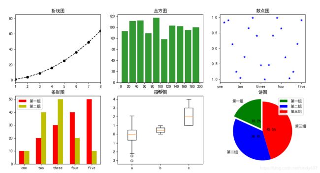
一、折线图

   import matplotlib.pyplot as plt
    import numpy as np
    import pandas as pd
    
    x = np.arange(1,10,1)
    y = x*x  # 创建数据
    fig= plt.figure(figsize=(20,40)) # 创建图片
    ax1 = fig.add_subplot(2,3,1)  # 创建子图
    plt.plot(x,y,'ko--')  # 在子图上画折线图，k是黑色，o是标记是圈，--是虚线
    plt.title('折线图')
    plt.xlim([1,8])  # 设置X刻度范围
    print(plt.ylim())  # 获取Y刻度范围
    plt.rcParams['font.sans-serif'] = ['SimHei']
    plt.rcParams['font.serif'] = ['SimHei']  # 设置正常显示中文
    plt.show()

二、直方图

'''调用的方法
matplotlib.pyplot.hist(
    x, 
    bins=None, #区间范围，如bins=[1, 2, 3, 4]，则第一个区间为[1,2)，第二个区间为[2,3)...依次类推
    range=None, 
    density=None, 
    weights=None, 
    cumulative=False, 
    bottom=None, #改变纵坐标基数，原纵坐标数值全部加上该基数
    histtype='bar', #{'bar'，'barstacked'，'step'，'stepfilled'}，可选
    align='mid', 
    orientation='vertical', #方向 {'horizo​​ntal'，'vertical'}
    rwidth=None, #矩形的宽度占区间的百分比，最大为1
    log=False, #如果为True，则直方图轴将被设置为对数刻度
    color=None, #直方图的颜色
    label=None, #直方图代表的名称
    stacked=False, #堆叠
    normed=None, #如果normed=True，则纵坐标数值会变，全部的矩形面积之和为1；
    hold=None, 
    data=None, 
    **kwargs
！'''
--------------------------------------
ax2 = fig.add_subplot(2,3,2)
y = np.random.randint(1,200,1000) # 随机生成1-199之间的1000个数
bins = [0,20,40,60,80,100,120,140,160,180,200]  # 分区间
plt.hist(y,bins=bins,rwidth=0.8,alpha=0.8,histtype='bar',color='g')  # bins是可以自己定区间，rwidth是宽度占的百分比
plt.xlabel('分区')
plt.xticks(bins)
plt.title('直方图')
plt.show()

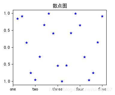
三、散点图

'''
matplotlib.pyplot.scatter(
    x, 
    y, 
    s=None, 
    c=None, 
    marker=None, 
    cmap=None, 
    norm=None, 
    vmin=None, 
    vmax=None, 
    alpha=None, 
    linewidths=None, 
    verts=None, 
    edgecolors=None, 
    hold=None, 
    data=None, 
    **kwargs
'''
--------------------------------------------------------
    x = np.linspace(1,20,20) # 按20/20为步长，生成1-20之间20个数
    y = np.sin(x)
    ax3 = fig.add_subplot(2,3,3)
    plt.scatter(x,y,linewidths=0.5,marker='*',color='b')
    ax3.set_xticks([0,5,10,15,20]) # 设置刻度
    ax3.set_xticklabels(['one','two','three','four','five']) #设置刻度展示
    plt.title('散点图')
    plt.show()

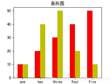
四、条形图

   '''
    bar(x, height, *, align='center', **kwargs)
    bar(x, height, width, *, align='center', **kwargs)
    bar(x, height, width, bottom, *, align='center', **kwargs)
    '''
    -------------------------------------------
        y1 = [10,20,30,40,50]
        y2 = [10,40,50,20,10]
        x=[1,2,3,4,5]
        bar_width=0.3  # 这个特别重要，可以确保两个条形图能仅仅挨在一起
        ax4 = fig.add_subplot(2,3,4)
        plt.bar(x=x, height=y1,label='第一组',color='r',width=bar_width)
        plt.bar(x=[i+bar_width for i in x], height=y2,label='第二组',width=bar_width,color='y') # x默认是在条形图的中间，加上bar_width/2就到了两个条形图的中间
        plt.xticks([i+bar_width/2 for i in x],['one','two','three','four','five'])  # 刻度也是一样调整到中间
        plt.title('条形图')
        plt.legend(loc='best')
        plt.show()

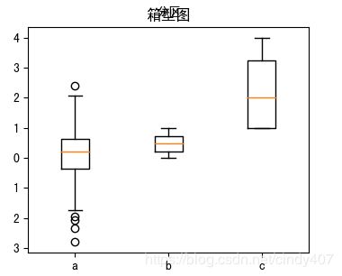
五、箱型图

ax5 = fig.add_subplot(2,3,5)
y1 = np.random.randn(100)
y2= np.random.random(100)
y3 = np.random.randint(1,5,100)
plt.boxplot((y1,y2,y3),labels=['a','b','c'])
plt.title('箱型图')
plt.show()

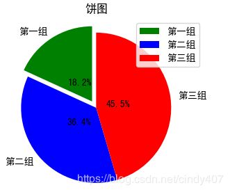
六、饼图

''' matplotlib.pyplot.pie(
    x, 
    explode=None, #突出的部分
    labels=None, #含义
    colors=None, #颜色
    autopct=None, 
    pctdistance=0.6, 
    shadow=False, #阴影
    labeldistance=1.1, 
    startangle=None, #开始的角度
    radius=None, #饼图半径
    counterclock=True, 
    wedgeprops=None, 
    textprops=None, 
    center=(0, 0), 
    frame=False, 
    hold=None, 
    data=None ) '''
    ---------------------------------

ax = fig.add_subplot(2,3,6)
    size = [20,40,50]
    lables=['第一组','第二组','第三组']
    colors=['green','blue','red']
    explode=[0.1,0,0]
    plt.pie(size,explode=explode,labels=lables,labeldistance=1.1,autopct='%1.1f%%',colors=colors,shadow=False,startangle=90,pctdistance=0.3)
    plt.legend(loc='best')
    plt.axis('equal')  # 坐标一致，才能是圆形
    plt.title('饼图')
    plt.show()

七、面积图

'''
stackplot(x, y)    # where y is MxN（2d array of dimension MxN）
stackplot(x, y1, y2, y3, y4)  # where y1, y2, y3, y4, are all 1xNm
stackplot(x, y1, y2, y3, y4, labels=[], colors=[])  
'''
------------------------------------------------
    plt.figure()
    x = [1,2,3,4,5]
    y1 = [12,34,54,23,54]
    y2 = [56,23,12,54,2]
    y3 = [12,43,54,23,54]
    plt.stackplot(x,y1,y2,y3,labels=['第一组','第二组','第三组','第四组'],colors=['r','g','k','y'])
    plt.title('面积图')
    plt.show()

---

本人互联网数据分析师，目前已出Excel，SQL，Pandas，Matplotlib，Seaborn，机器学习，统计学，个性推荐，关联算法，工作总结系列。

---

微信搜索并关注 " 数据小斑马" 公众号，回复“数据分析”可以免费获取下方15本数据分析师必备学习书籍一套