教程2：Matlab图像处理基础（二）

自己学习SVD的主要概念，同时学习图像滤波，完成下面作业：

作业1： Image Manipulation

(a) The provided ImageManip.m script reads in the provided u2dark.png photo and converts it to grayscale using rgb2gray. Use the script and your own code to calculate the following statistics: What is the average pixel vale of the resulting grayscale image? What are the min and max values? (There are several ways to calculate these quantities in MATLAB. Review the MATLAB tutorial if you need help.)

(b) We would like to bring the image to a more typical brightness. Add an offset and apply a scaling factor to all pixels, so that the minimum pixel value becomes 0 and the max pixel value becomes 255. (Cameras often do a similar function automatically.) Include the final image in your report, as well as the MATLAB code you used to produce it.

© Next, we would like to double the contrast of the pixels in the middle brightness range. Specifically, take your rest from part (b) and replace each pixel’s intensity $i$ with a new intensity $i’$, where
$$i^{\prime }=2\ast (i-128)+128$$
Thereshold $i^{\prime }$ so that $0\le i^{\prime }\le 255$ (you can use the uint8 function). Include your MATLAB code and the resulting contrast-boosted image in your report. Compare the image ot part (b). What was the downside of increasing contrast in this way, and why did it happen?

imageManip.m

%reads in the image, converts it to grayscale, and converts the intensities
%from uint8 integers to doubles. (Brightness must be in 'double' format for
%computations, or else MATLAB will do integer math, which we don't want.)
dark = double(rgb2gray(imread('u2dark.png')));

%%%%%% Your part (a) code here: calculate statistics

%%%%%% Your part (b) code here: apply offset and scaling
fixedimg = [];

%displays the image
imshow(uint8(fixedimg));

%%%%%% Your part (c) code here: apply the formula to increase contrast,
% and display the image
contrasted = [];

作业2： Edge Detection

An “edge” is a place where image intensity changes abruptly. Edges can indicate the borders of objects.

(a) The intensity changes associated with vertical edges can be detected by calculating:
$$horizontalgradient\approx (thepixel)-(pixelonitsleft)$$
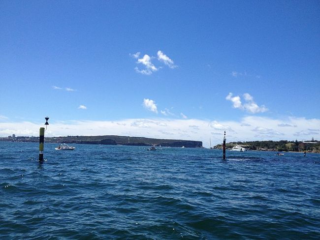
for every pixel in the image. Open edgedetector.m and edit the DetectVerticalEdges() function to do this. Run the edgedetector() function to display your calculated gradients as an image. Compare the original image to the image of gradients. Veryfy that the vertical edges were detected and are visible as very bright / dark spots that indicate “edges” in the water. What caused these tiny “edges”?

(b) We will now assess the effects of “blurring” the gradient image. The simplest blurring operation is the box blur. In a box of width $n$, each blurred pixel is computed as follows:
$$blur(x,y)=\frac{1}{n^2}\sum _{i=0}^{n-1}\sum _{j=0}^{n-1}img(x+i,y+j)$$
In edgedetector.m , edit the BoxBlur() function to do this, and run the edgedetector() function to veiw the results. What was the effect of the blur on the large edges, compared to the tiny “noise” edges? Why?

% This function calls the functions below and displays their results.
% You don't need to edit it.
function edgedetector()
    img = double(rgb2gray(imread('buoys.jpg')));

    edges = DetectVerticalEdges(img);
    blurred_edges = BoxBlur(edges);
    
    figure('Name','Original Image')
    imshow(img, []);
    
    figure('Name','Edges')
    imshow(edges, []);
    
    
    figure('Name','Blurred Edges')
    imshow(blurred_edges, []);
end


% Returns a matrix containing the horizontal component of the gradient at every
% image location.
function edges = DetectVerticalEdges(img)
    % MATLAB images use matrix indices, so the order is (y,x), and the +y
    % direction is downward.
    width = size(img, 2);
    height = size(img, 1);
    
    %%%%%%%%%%%%%%%%%%%%%%%%%%%%%%%%%%%%%%%%%%%%%%%%%%%%%%%%%%%%%%%%%%%
    %%%%%%%%%% Your part (a) code here. You can accomplish part (a) with
    %%%%%%%%%% nested "for" loops, but an easier way is to use matrix 
    %%%%%%%%%% indexing to make a matrix of the "left" pixels and a matrix 
    %%%%%%%%%% of the "right" pixels, and subtract the two matrices.
    %%%%%%%%%% REMEMBER: left/right position is the SECOND index in MATLAB.
    edges = zeros(height, width-1);
    
    %%%%%%%%%% End of your part (a) code.
end

% Applies a box blur to the input image and returns the result.
function blurred = BoxBlur(img)
    img = double(img);

    height = size(img, 1);
    width = size(img, 2);
    n=5; % width of the blur
    blurred = zeros(height-(n-1),width-(n-1));
    % Loop through each pixel location in the result
    for y=1:height-(n-1)
        for x=1:width-(n-1)
            %%%%%%%%%%%%%%%%%%%%%%%%%%%%%%%%%%%%%%%%%%%%%%%%%%%%%%%
            %%%%%%% Your part (b) code here. Calculate blurred(y,x).
            
            %%%%%%% End of part (b) code
        end
    end
    
    % Usually we'll divide at the end so that we don't make the image
    % brighter:
    blurred = blurred / n^2;    
end

作业3： SVD for Image Compression

Singular value decomposition (SVD) can be effectively used to compress images. Suppose $I$ is the pixel intensity matrix of a large image $n\times n$. The transmission of $I$ requires $O(n^2)$ numbers. Instead, one could use $I_k$, that is, the top $k$ signular values ${\sigma }_1,{\sigma }_2,\dots ,{\sigma }_k$ along with the left and right singular vectors $u_1,u_2,\dots ,u_k$ and $v_1,v_2,\dots ,v_k$. This would require using $O(kn)$ real numbers instead of $O(n^2)$ real numbers. If $k$ is much smaller than $n$, this results in substantial savings.

In this problem, you will explore SVD compression on the flower.bmp image we have provided. In addition to your answers to each question, you should also submit your MATLAB code and reqiured plots where necessary. Hint: You may find the MATLAB svd command particularly useful for this problem.

(a) Use MATLAB to read in flower.bmp and convert it to grayscale and “double” format. Apply SVD and give the top 10 singular values. Generate a plot for all singular values versus their rankings (the diag command may be helpful to format the values). What do you notice from this plot?

(b) Verify that you can reconstruct and display the image using the three SVD matrices (note that the svd command returns $V$, not $V^T$). Then, perform compression by using only the top $k$ singular values and their corresponding left / right singular vectors. Let $k$ = 10, 50, and 100. Reconstruct and print the compressed images for the three different values of $k$. Briefly describe what you observe.

需要用到的图片：

buoys.jpg

u2dark.jpg

flower.jpg