《Machine Learning（Tom M. Mitchell）》读书笔记——7、第六章

1. Introduction (about machine learning)

2. Concept Learning and the General-to-Specific Ordering

3. Decision Tree Learning

4. Artificial Neural Networks

5. Evaluating Hypotheses

6. Bayesian Learning

7. Computational Learning Theory

8. Instance-Based Learning

9. Genetic Algorithms

10. Learning Sets of Rules

11. Analytical Learning

12. Combining Inductive and Analytical Learning

13. Reinforcement Learning

6. Bayesian Learnin

6.1 INTRODUCTION

Bayesian learning methods are relevant to our study of machine learning for two different reasons.  First, Bayesian learning algorithms that calculate explicit probabilities for hypotheses, such as the naive Bayes classifier(朴素贝叶斯分类器), are among the most practical approaches to certain types of learning problems.  The second reason that Bayesian methods are important to our study of machine learning is that they provide a useful perspective for understanding many learning algorithms that do not explicitly manipulate probabilities. 

One practical difficulty in applying Bayesian methods is that they typically require initial knowledge of many probabilities. When these probabilities are not known in advance they are often estimated based on background knowledge, previously available data, and assumptions about the form of the underlying distributions. A second practical difficulty is the significant computational cost required to determine the Bayes optimal hypothesis in the general case (linear in the number of candidate hypotheses). 

6.2 BAYES THEOREM 

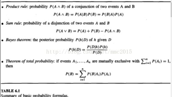
作为理科生，概率论是基础，就不细说了！

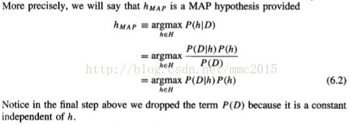
The most probable hypothesis h ∈ H given the observed data D (or at least one of the maximally probable if there are several)  is called a maximum a posteriori (MAP) hypothesis(极大后验假设).

We will assume that every hypothesis in H is equally probable a priori (P(hi) = P(hj) for all hi and hj in H). In this case we can further simplify Equation (6.2) and need only consider the term P(D|h) to find the most probable hypothesis.

极大似然假设

6.3 BAYES THEOREM AND CONCEPT LEARNING

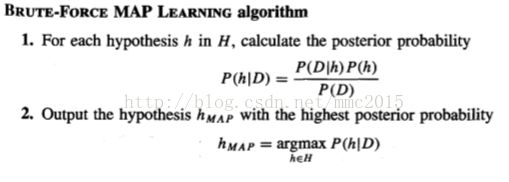
6.3.1 Brute-Force Bayes Concept Learning 

This algorithm may require significant computation, because it applies Bayes theorem to each hypothesis in H to calculate P(hJ D). While this may prove impractical for large hypothesis spaces, the algorithm is still of interest because it provides a standard against which we may judge the performance of other concept learning algorithms.

(推导过程略)

where

, because  every hypothesis h in H has the same prior probability;

, because we assume noise-free training data, the probability of observing classification di given h is just 1 if di = h(xi) and 0 if di != h(xi).

6.3.2 MAP Hypotheses and Consistent Learners(极大后验假设和一致学习器，这两者在一定条件下是等价的)

We will say that a learning algorithm is a consistent learner provided it outputs a hypothesis that commits zero errors over the training examples. Given the above analysis, we can conclude that every consistent learner outputs a MAP hypothesis, if we assume a uniform prior probability distribution over H (i.e., P(hi) = P(hj) for all i, j), and ifwe assume deterministic, noise free training data (i.e., P(D Ih) = 1 if D and h are consistent, and 0 otherwise).

To summarize, the Bayesian framework allows one way to characterize the behavior of learning algorithms (e.g., FIND-S),e ven when the learning algorithm does not explicitly manipulate probabilities. By identifying probability distributions P(h) and P(Dlh) under which the algorithm outputs optimal (i.e., MAP) hypotheses, we can characterize the implicit assumptions , under which this algorithm behaves optimally. 

6.4 MAXIMUM LIKELIHOOD AND LEAST-SQUARED ERROR HYPOTHESES(极大似然假设和最小误差平方假设，这两者在一定条件下是等价的)

A straightforward Bayesian analysis will show that under certain assumptions any learning algorithm that minimizes the squared error between the output hypothesis predictions and the training data will output a maximum likelihood hypothesis.

P165-P166应用probability densities and Normal distributions的相关性质推到了一个关系式：

.

Thus, Equation (6.6) shows that the maximum likelihood hypothesis hML is the one that minimizes the sum of the squared errors between the observed training values di and the hypothesis predictions h(xi). This holds under the assumption that the observed training values di are generated by adding random noise to the true target value, where this random noise is drawn independently for each example from a Normal distribution with zero mean. 

Of course, the maximum likelihood hypothesis might not be the MAP hypothesis, but if one assumes uniform prior probabilities over the hypotheses then it is.

6.5 MAXIMUM LIKELIHOOD HYPOTHESES FOR PREDICTING PROBABILITIES 

In this section we derive a weight-training rule for neural network learning that seeks to maximize G(h, D) using gradient ascent. 

作为理科生，数学是基础，就不细说了！

To summarize section 6.4 and section 6.5, these two weight update rules converge toward maximum likelihood hypotheses in two different settings. The rule that minimizes sum of squared error seeks the maximum likelihood hypothesis under the assumption that the training data can be modeled by Normally distributed noise added to the target function value. The rule that minimizes cross entropy(交叉熵) seeks the maximum likelihood hypothesis under the assumption that the observed boolean value is a probabilistic function of the input instance. 

6.6 MINIMUM DESCRIPTION LENGTH PRINCIPLE

Clearly, to minimize the expected code length we should assign shorter codes to messages that are more probable. Shannon and Weaver (1949) showed that the optimal code (i.e., the code that minimizes the expected message length) assigns -log2pi bits to encode message i. We will refer to the number of bits required to encode message i using code C as the description length of message i with respect to C, which we denote by Lc(i). 

6.7 BAYES OPTIMAL CLASSIFIER(贝叶斯最优分类器)

No other classification method using the same hypothesis space and same prior knowledge can outperform this method on average. This method maximizes the probability that the new instance is classified correctly, given the available data, hypothesis space, and prior probabilities over the hypotheses.

Note one curious property of the Bayes optimal classifier is that the pre- dictions it makes can correspond to a hypothesis not contained in H! One way to view this situation is to think of the Bayes optimal classifier as effectively considering a hypothesis space H' different from the space of hypotheses H to which Bayes theorem is being applied. In particular, H' effectively includes hypotheses that perform comparisons between linear combinations of predictions from multiple hypotheses in H. 

6.8 GIBBS ALGORITHM

In particular, it implies that if the learner assumes a uniform prior over H, and if target concepts are in fact drawn from such a distribution when presented to the learner, then classifying the next instance according to a hypothesis drawn at random from the current version space (according to a uniform distribution), will have expected error at most twice that of the Bayes optimal classijier. Again, we have an example where a Bayesian analysis of a non-Bayesian algorithm yields insight into the performance of that algorithm. 

6.9 NAIVE BAYES CLASSIFIER(朴素贝叶斯分类器)

The naive Bayes classifier applies to learning tasks where each instance x is described by a conjunction of attribute values and where the target function f (x) can take on any value from some finite set V. A set of training examples of the target function is provided, and a new instance is presented, described by the tuple of attribute values (al, a2.. .a,). The learner is asked to predict the target value, or classification, for this new instance. 

The Bayesian approach:

The problem is that the number of these terms(different P(al, a2.. an | vj) terms) is equal to the number of possible instances times the number of possible target values. Therefore, we need to see every instance in the instance space many times in order to obtain reliable estimates.

The naive Bayes classifier is based on the simplifying assumption that the attribute values are conditionally independent(条件独立) given the target value. 

 Whenever the naive Bayes assumption of conditional independence is satisfied, this naive Bayes classification VNB is identical to the MAP classification.

Notice that in a naive Bayes classifier the number of distinct P(ai l vj) terms that must be estimated from the training data is just the number of distinct attribute values times the number of distinct target values-a much smaller number than if we were to estimate the P(a1, a2 . . . an l vj) terms as first contemplated.

6.10 AN EXAMPLE: LEARNING TO CLASSIFY TEXT

6.11 BAYESIAN BELIEF NETWORKS 

In this section we introduce the key concepts and the representation of Bayesian belief networks.

Consider an arbitrary set of random variables Y1 . . . Yn, where each variable Yi can take on the set of possible values V(Yi). We define the joint space(联合空间) of the set of variables Y to be the cross product(叉乘) V(Y1) x V(Y2) x . . . V(Yn). In other words, each item in the joint space corresponds to one of the possible assignments of values to the tuple of variables (Y1 . . . Yn). The probability distribution over this joint space is called the joint probability distribution(联合概率分布). A Bayesian belief network describes the joint probability distribution for a set of variables. 

6.11.1 Conditional Independenc

概率论，不细说

6.11.2 Representation

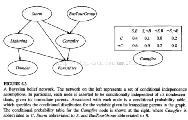
In general, a Bayesian network represents the joint probability distribution by specifying a set of conditional independence assumptions(条件独立假设, represented by a directed acyclic graph), together with sets of local conditional probabilities(局部条件概率). Each variable in the joint space is represented by a node in the Bayesian network. For each variable two types of information are specified, the network arcs and a conditional probability table.

The joint probability for any desired assignment of values (y1, . . . , yn) to the tuple of network variables (Y1 . . . Yn) can be computed by the formula 

6.11.3 Inference

In general, a Bayesian network can be used to compute the probability distribution for any subset of network variables given the values or distributions for any subset of the remaining variables.

Exact inference of probabilities in general for an arbitrary Bayesian network is known to be NP-hard (Cooper 1990). Numerous methods have been proposed for probabilistic inference in Bayesian networks, including exact inference methods and approximate inference methods that sacrifice precision to gain efficiency. For example, Monte Carlo methods provide approximate solutions by randomly sampling the distributions of the unobserved variables (Pradham and Dagum 1996).

6.11.4 Learning Bayesian Belief Networks

In the case where the network structure is given in advance and the variables are fully observable in the training examples, learning the conditional probability tables is straightforward. We simply estimate the conditional probability table entries just as we would for a naive Bayes classifier.

In the case where the network structure is given but only some of the variable values are observable in the training data, the learning problem is more difficult......6.11.5....

6.11.5 Gradient Ascent Training of Bayesian Networks 

P188-P190

6.11.6 Learning the Structure of Bayesian Networks

Learning Bayesian networks when the network structure is not known in advance is also difficult.

6.12 THE EM ALGORITHM

In this section we describe the EM algorithm (Dempster et al. 1977), a widely used approach to learning in the presence of unobserved variables. The EM algorithm can be used even for variables whose value is never directly observed, provided the general form of the probability distribution governing these variables is known.

6.12.1 Estimating Means of k Gaussians

6.12.2 General Statement of EM Algorithm

 More generally, the EM algorithm can be applied in many settings where we wish to estimate some set of parameters 8 that describe an underlying probability distribution, given only the observed portion of the full data produced by this distribution.

6.12.3 Derivation of the k Means Algorithm

P195-P196

6.13 SUMMARY AND FURTHER READING

Bayesian methods provide the basis for probabilistic learning methods that accommodate (and require) knowledge about the prior probabilities of alternative hypotheses and about the probability of observing various data given the hypothesis. Bayesian methods allow assigning a posterior probability to each candidate hypothesis, based on these assumed priors and the observed data. 

Bayesian methods can be used to determine the most probable hypothesis given the data-the maximum a posteriori (MAP) hypothesis. This is the optimal hypothesis in the sense that no other hypothesis is more likely. 

The Bayes optimal classifier combines the predictions of all alternative hypotheses, weighted by their posterior probabilities, to calculate the most probable classification of each new instance.

The naive Bayes classifier is a Bayesian learning method that has been found to be useful in many practical applications. It is called "naive" because it incorporates the simplifying assumption that attribute values are conditionally independent, given the classification of the instance. When this assumption is met, the naive Bayes classifier outputs the MAP classification. Even when this assumption is not met, as in the case of learning to classify text, the naive Bayes classifier is often quite effective. Bayesian belief networks provide a more expressive representation for sets of conditional independence assumptions among subsets of the attributes. 

The framework of Bayesian reasoning can provide a useful basis for analyzing certain learning methods that do not directly apply Bayes theorem. For example, under certain conditions it can be shown that minimizing the squared error when learning a real-valued target function corresponds to computing the maximum likelihood hypothesis. 

The Minimum Description Length principle recommends choosing the hypothesis that minimizes the description length of the hypothesis plus the description length of the data given the hypothesis. Bayes theorem and basic results from information theory can be used to provide a rationale for this principle. 

In many practical learning tasks, some of the relevant instance variables may be unobservable. The EM algorithm provides a quite general approach to learning in the presence of unobservable variables. This algorithm begins with an arbitrary initial hypothesis. It then repeatedly calculates the expected values of the hidden variables (assuming the current hypothesis is correct), and then recalculates the maximum likelihood hypothesis (assuming the hidden variables have the expected values calculated by the first step). This procedure converges to a local maximum likelihood hypothesis, along with estimated values for the hidden variables.