李理：三层卷积网络和vgg的实现

本系列文章面向深度学习研发者，希望通过Image Caption Generation，一个有意思的具体任务，深入浅出地介绍深度学习的知识。本系列文章涉及到很多深度学习流行的模型，如CNN，RNN/LSTM，Attention等。本文为第12篇。

作者：李理
目前就职于环信，即时通讯云平台和全媒体智能客服平台，在环信从事智能客服和智能机器人相关工作，致力于用深度学习来提高智能机器人的性能。

相关文章：
李理：从Image Caption Generation理解深度学习（part I）
李理：从Image Caption Generation理解深度学习（part II）
李理：从Image Caption Generation理解深度学习（part III）
李理：自动梯度求解 反向传播算法的另外一种视角
李理：自动梯度求解——cs231n的notes
李理：自动梯度求解——使用自动求导实现多层神经网络
李理：详解卷积神经网络
李理：Theano tutorial和卷积神经网络的Theano实现 Part1
李理：Theano tutorial和卷积神经网络的Theano实现 Part2
李理：卷积神经网络之Batch Normalization的原理及实现
李理：卷积神经网络之Dropout

卷积神经网络的原理已经在《李理：卷积神经网络之Batch Normalization的原理及实现》以及《李理：卷积神经网络之Dropout》二文中详细讲过了，这里我们看怎么实现。

5.1 cell1-2

打开ConvolutionalNetworks.ipynb，运行cell1和2

5.2 cell3 实现最原始的卷积层的forward部分

打开layers.py，实现conv_forward_naive里的缺失代码：

N, C, H, W = x.shape
  F, _, HH, WW = w.shape
  stride = conv_param['stride']
  pad = conv_param['pad']
  H_out = 1 + (H + 2 * pad - HH) / stride
  W_out = 1 + (W + 2 * pad - WW) / stride
  out = np.zeros((N,F,H_out,W_out))

  # Pad the input
  x_pad = np.zeros((N,C,H+2*pad,W+2*pad))
  for n in range(N):
    for c in range(C):
      x_pad[n,c] = np.pad(x[n,c],(pad,pad),'constant', constant_values=(0,0))

  for n in range(N):
      for i in range(H_out):
        for j in range(W_out):
          current_x_matrix = x_pad[n, :, i * stride: i * stride + HH, j * stride:j * stride + WW]
          for f in range(F):
            current_filter = w[f]
            out[n,f,i,j] = np.sum(current_x_matrix*current_filter)

          out[n,:,i,j] = out[n,:,i,j]+b

我们来逐行来阅读上面的代码

5.2.1 第1行

首先输入x的shape是(N, C, H, W)，N是batchSize，C是输入的channel数，H和W是输入的Height和Width

5.2.2 第2行

参数w的shape是(F, C, HH, WW)，F是Filter的个数，HH是Filter的Height，WW是Filter的Width

5.2.3 第3-4行

从conv_param里读取stride和pad

5.2.4 第5-6行

计算输出的H_out和W_out

5.2.5 第7行

定义输出的变量out，它的shape是(N, F, H_out, W_out)

5.2.6 第8-11行

对x进行padding，所谓的padding，就是在一个矩阵的四角补充0。

首先我们来熟悉一下numpy.pad这个函数。

In [19]: x=np.array([[1,2],[3,4],[5,6]])

In [20]: x
Out[20]: 
array([[1, 2],
       [3, 4],
       [5, 6]])

首先我们定义一个3*2的矩阵

然后给它左上和右下都padding1个0。

In [21]: y=np.pad(x,(1,1),'constant', constant_values=(0,0))

In [22]: y
Out[22]: 
array([[0, 0, 0, 0],
       [0, 1, 2, 0],
       [0, 3, 4, 0],
       [0, 5, 6, 0],
       [0, 0, 0, 0]])

我们看到3*2的矩阵的上下左右都补了一个0。

我们也可以只给左上补0：

In [23]: y=np.pad(x,(1,0),'constant', constant_values=(0,0))

In [24]: y
Out[24]: 
array([[0, 0, 0],
       [0, 1, 2],
       [0, 3, 4],
       [0, 5, 6]])

了解了pad函数之后，上面的代码就很容易阅读了。对于每一个样本，对于每一个channel，这都是一个二位的数组，我们根据参数pad对它进行padding。

5.2.7 第12-19行

这几行代码就是按照卷积的定义：对于输出的每一个样本(for n in range(N))，对于输出的每一个下标i和j，我们遍历所有F个filter，首先找到要计算的局部感知域：

current_x_matrix = x_pad[n,:, i*stride: i*stride+HH, j*stride:j*stride+WW]

这会得到一个(C, HH, WW)的ndarray，也就是下标i和j对应的。

然后我们把这个filter的参数都拿出来：

current_filter = w[f]

它也是(C, HH, WW)的ndarray。

然后对应下标乘起来，最后加起来。

如果最简单的实现，我们还应该加上bias

out[n,f,i,j]+=b[f]

这也是可以的，但是为了提高运算速度，我们可以把所有filter的bias一次用向量加法实现，也就是上面代码的方式。

其中烦琐的地方就是怎么通过slice得到当前的current_x_matrix。不清楚的地方可以参考下图：

关于上面的4个for循环，其实还有一种等价而且看起来更自然的实现：

  for n in range(N):
    for f in range(F):
      current_filter = w[f]
      for i in range(H_out):
        for j in range(W_out):
          current_x_matrix = x_pad[n, :, i * stride: i * stride + HH, j * stride:j * stride + WW]
          out[n, f, i, j] = np.sum(current_x_matrix * current_filter)
          out[n, f, i, j] = out[n, f, i, j] + b[f]

为什么不用这种方式呢？

首先这种方式bias没有办法写出向量的形式了，其次我觉得最大的问题是切片操作次数太多，对于这种方式，current_x_matrix从x_pad切片的调用次数是N F H_out*W_out。切片会访问不连续的内存，这是会极大影响性能的。

5.3 cell4

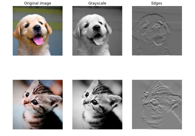
通过卷积实现图像处理。

这个cell通过卷积来进行图像处理，实现到灰度图的转化和边缘检测。这一方面可以验证我们之前的算法，另外也可以演示卷积可以提取一些特征。

实现灰度图比较简单，每个像素都是 gray=r∗0.1+b∗0.6+g∗0.3
用一个卷积来实现就是：

w[0, 0, :, :] = [[0, 0, 0], [0, 0.3, 0], [0, 0, 0]]
w[0, 1, :, :] = [[0, 0, 0], [0, 0.6, 0], [0, 0, 0]]
w[0, 2, :, :] = [[0, 0, 0], [0, 0.1, 0], [0, 0, 0]]

而下面的filter是一个sobel算子，用来检测水平的边缘：

w[1, 0, :, :] =0
w[1, 1, :, :] =0
w[1, 2, :, :] = [[1, 2, 1], [0, 0, 0], [-1, -2, -1]]

感兴趣的读者可以参考 sobel operator
读者可能问了，这么做有什么意义？这个例子想说明的是卷积能够做一些图像处理的事情，而通过数据的驱动，是可以(可能)学习出这样的特征的。而在深度学习之前，很多时候是人工在提取这些特征。以前做图像识别，需要很多这样的算子，需要很多图像处理的技术，而现在就不需要那么多了。

这个cell不需要实现什么代码，直接运行就好了。

5.4 cell5 实现conv_backward_naive

代码如下：

  x, w, b, conv_param = cache
  stride = conv_param['stride']
  pad = conv_param['pad']
  N, C, H, W = x.shape
  F, _, HH, WW = w.shape
  _,_,H_out,W_out = dout.shape

  x_pad = np.zeros((N,C,H+2*pad,W+2*pad))
  for n in range(N):
    for c in range(C):
      x_pad[n,c] = np.pad(x[n,c],(pad,pad),'constant', constant_values=(0,0))

  db = np.zeros((F))

  dw = np.zeros(w.shape)
  dx_pad = np.zeros(x_pad.shape)

  for n in range(N):
    for i in range(H_out):
      for j in range(W_out):
        current_x_matrix = x_pad[n, :, i * stride: i * stride + HH, j * stride:j * stride + WW]
        for f in range(F):
          dw[f] = dw[f] + dout[n,f,i,j]* current_x_matrix
          dx_pad[n,:, i*stride: i*stride+HH, j*stride:j*stride+WW] += w[f]*dout[n,f,i,j]
        db = db + dout[n,:,i,j]
  dx = dx_pad[:,:,pad:H+pad,pad:W+pad]

代码和forward很像，首先是把cache里的值取出来。由于x_pad没有放到cache里，这里还需要算一遍，当然也可以修改上面的forward，这样避免padding。

然后定义db,dw,dx_pad

最后是和forward完全一样的一个4层for循环，区别是：

    #forward
    current_x_matrix = x_pad[n, :, i * stride: i * stride + HH, j * stride:j * stride + WW]
        out[n,f,i,j] = np.sum(current_x_matrix* w[f])
       #backward
       dw[f] += dout[n,f,i,j]*current_x_matrix
       dx_pad[....]+=dout * w[f]

这里的小小技巧就是 z=np.sum(matrix1*matrix2)，怎么求dz/dmatrix1。
答案就是matrix2。

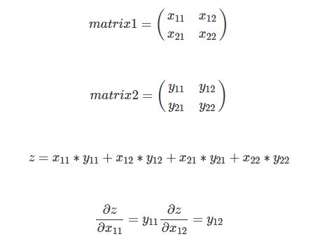
所以写出矩阵的形式就是dz/matrix1=matrix2。

我们运行一下这个cell，如果相对误差小于10的-9次方，那么我们的实现就是没有问题的。

5.5 cell6 实现max_pool_forward_naive

  N, C, H, W = x.shape
  pool_height = pool_param['pool_height']
  pool_width = pool_param['pool_width']
  stride = pool_param['stride']
  H_out = 1 + (H - pool_height) / stride
  W_out = 1 + (W - pool_width) / stride
  out = np.zeros((N,C,H_out,W_out))

  for n in range(N):
    for c in range(C):
      for h in range(H_out):
        for w in range(W_out):
          out[n,c,h,w] = np.max(x[n,c, h*stride:h*stride+pool_height, w*stride:w*stride+pool_width])

max_pool的forward非常简单，就是在对应的局部感知域里选择最大的那个数就行。

5.6 cell7 实现max_pool_backward_naive

  x, pool_param = cache
  pool_height = pool_param['pool_height']
  pool_width = pool_param['pool_width']
  stride = pool_param['stride']
  N, C, H_out, W_out = dout.shape

  dx = np.zeros(x.shape)

  for n in range(N):
    for c in range(C):
      for h in range(H_out):
        for w in range(W_out):
          current_matrix = x[n, c, h * stride:h * stride + pool_height, w * stride:w * stride + pool_width]
          max_idx = np.unravel_index(np.argmax(current_matrix),current_matrix.shape)
          dx[n, c, h * stride + max_idx[0], w * stride + max_idx[1]] += dout[n, c, h, w]

backward也很简单，就是最大的局部感知域最大的那个dx是1，其余的是0。为了提高效率，其实forward阶段是可以”记下“最大的那个下标，这里是重新计算的。

稍微注意一下就是np.argmax返回的是最大的下标，是把2维数组展开成一维的下标，为了变成二维数组的下标，我们需要用unravel_index这个函数。

In [3]: x
Out[3]: 
array([[1, 2, 3],
       [4, 5, 6]])

In [5]: x.argmax()
Out[5]: 5

In [6]: ind = np.unravel_index(np.argmax(x),x.shape)

In [7]: ind
Out[7]: (1, 2)

5.7 cell8-9

作业提供了卷积和pooling的加速实现，它里面已经实现好了，我们这里就不再讲解其实现细节了，有兴趣的读者可以参考作业的代码以及参考 http://cs231n.stanford.edu/slides/winter1516_lecture11.pdf 的im2col部分。

这里只是比较了它们的速度

卷积的快速版本和原始版本比较

pooling的快速版本和原始版本比较

5.8 cell10-11

把卷积，pooling和relu组装在一起，代码已经实现，直接执行验证一下就好了

5.9 cell12 三层的卷积神经网络

打开cs231n/cnn.py实现ThreeLayerConvNet

首先我们来看看这个网络的结构：

conv - relu - 2x2 max pool - affine - relu - affine - softmax

这个网络有三层，第一层是卷积-relu激活-max pooling。第二层是全连接层affine-relu激活，第三层是线性的affine加softmax

5.9.1 init函数

这个函数定义了网络的输入维度，卷积的filter个数，卷积的大小，全连接层隐单元个数，输出维度等。请仔细阅读代码中的注释。

  def __init__(self, input_dim=(3, 32, 32), num_filters=32, filter_size=7,
               hidden_dim=100, num_classes=10, weight_scale=1e-3, reg=0.0,
               dtype=np.float32):
    """
    初始化一个新的网络

    输入:
    - input_dim: 三元组 (C, H, W) 给定输入的Channel数，Height和Width
    - num_filters: 卷积层的filter的个数（feature map）
    - filter_size: filter的width和height，这里假设是一样的。
    - hidden_dim: 全连接层hidden unit的个数
    - num_classes: 输出的类别数
    - weight_scale: 初始化weight高斯分布的标准差

    - reg: L2正则化系数
    - dtype: 浮点数的类型
    """
    self.params = {}
    self.reg = reg
    self.dtype = dtype

    ############################################################################
    # TODO: Initialize weights and biases for the three-layer convolutional    #
    # network. Weights should be initialized from a Gaussian with standard     #
    # deviation equal to weight_scale; biases should be initialized to zero.   #
    # All weights and biases should be stored in the dictionary self.params.   #
    # Store weights and biases for the convolutional layer using the keys 'W1' #
    # and 'b1'; use keys 'W2' and 'b2' for the weights and biases of the       #
    # hidden affine layer, and keys 'W3' and 'b3' for the weights and biases   #
    # of the output affine layer.                                              #
    ############################################################################
    C, H, W = input_dim
    self.params['W1'] = np.random.normal(0, weight_scale, (num_filters, C, filter_size, filter_size))
    self.params['b1'] = np.zeros(num_filters)

    self.params['W2'] = np.random.normal(0, weight_scale, (num_filters*H/2*W/2, hidden_dim))
    self.params['b2'] = np.zeros(hidden_dim)

    self.params['W3'] = np.random.normal(0, weight_scale, (hidden_dim, num_classes))
    self.params['b3'] = np.zeros(num_classes)

    ############################################################################
    #                             END OF YOUR CODE                             #
    ############################################################################

    for k, v in self.params.iteritems():
      self.params[k] = v.astype(dtype)

init主要的代码就是初始化三层卷积网络的参数W和b。

• W1的shape是(num_filters, C, filter_size, filter_size)
• b1的shape是(num_filters)
• W2的shape是(num_filters H/2 w/2, hidden_dim)，因为(C, H, W)经过卷积后变成(num_filters, H, W)【这里使用的padding方法使得输出的H和W保持不变】，在经过pooling后H，W减半【这里的pooling没有padding，2*2 pooling，stride是2】
• b2的shape是(hidden_dim)
• W3的shape是(hidden_dim, num_classes)
• b3是(num_classes)

5.9.2 loss函数

在ThreeLayerConvNet类里，我们把predict和loss合并成了一个函数。如果输入y不是None，我们就认为是loss，否则只进行forward部分【loss也要forward】，区别在于predict没有必要计算softmax，只需要计算最好一个affine就行了，原因是softmax是单调的，计算softmax后再挑选最大的那个下标和不计算softmax是一样的。

1. forward部分

    conv_out, conv_cache = conv_forward_fast(X, W1, b1, conv_param)
    relu1_out, relu1_cache = relu_forward(conv_out)
    pool_out, pool_cache = max_pool_forward_fast(relu1_out, pool_param)
    affine_relu_out, affine_relu_cache = affine_relu_forward(pool_out, W2, b2)
    affine2_out, affine2_cache = affine_forward(affine_relu_out, W3, b3)
    scores = affine2_out

代码非常简单：

• 第一行是进行卷积，同时要保存cache，后面backward会用到
• 第二行是relu
• 第三行是max_pool
• 第四行是affine_relu，把affine和relu同时做了，当然分开也是可以的。
• 第五行是affine

    if y is None:
      return scores

接下来判断y是否None【也就是test还是train阶段】

2. backwoard

    loss, dscores = softmax_loss(scores, y)
    loss += 0.5 * self.reg*(np.sum(self.params['W1']* self.params['W1'])
         + np.sum(self.params['W2']* self.params['W2'])
         + np.sum(self.params['W3']* self.params['W3']))

    affine2_dx, affine2_dw, affine2_db = affine_backward(dscores, affine2_cache)
    grads['W3'] = affine2_dw + self.reg * self.params['W3']
    grads['b3'] = affine2_db

    affine1_dx, affine1_dw, affine1_db = affine_relu_backward(affine2_dx, affine_relu_cache)

    grads['W2'] = affine1_dw + self.reg * self.params['W2']
    grads['b2'] = affine1_db

    pool_dx = max_pool_backward_fast(affine1_dx, pool_cache)
    relu_dx = relu_backward(pool_dx, relu1_cache)
    conv_dx, conv_dw, conv_db = conv_backward_fast(relu_dx, conv_cache)
    grads['W1'] = conv_dw + self.reg * self.params['W1']
    grads['b1'] = conv_db

首先是调用softmax_loss函数
这个函数输入是最后一个affine的输出score和y计算出loss以及 ∂Loss/∂score
然后loss记得加上L2正则化的部分

接下来的步骤就非常”机械“和简单了。
我们之 需要把forward的每个函数调用对应的back函数，
比如我们最后一句forward是：

affine2_out, affine2_cache = affine_forward(affine_relu_out, W3, b3)

那么对应的backward就是：

affine2_dx, affine2_dw, affine2_db = affine_backward(dscores, affine2_cache)

基本的”模板“就是

out, cache=xxx_forward(x,y,z)
dx,dy,dz=xxx_backward(dout, cache)

这里就不一一赘述细节了，有了dx，那么就可以把它保存到grads[‘x’]里，注意weight有正则化项 reg∗x² ，所以对x求导后还剩下 2∗reg∗x，也要记得更新到grad[‘x’]里去。

5.10 cell13-14 sanity check和gradient check

我们的代码写完了，怎么验证forward和backward呢？我们知道可以用数值梯度来验证梯度，所以这个还比较容易验证，那么forwar呢？之前的作业老师都准备好了一下单元测试的例子，给定x和y，我们实现的forward就是要通过x计算出y来。

但是如果我们自己设计一个网络，没有”参考答案”怎么验证呢？当然没法绝对的验证，但是可以做“sanity check”。什么意思？对于随机初始化的参数，我们让模型来分类，那么它应该是“乱猜”的，比如分类数是10，那么它分类的准确率应该是10%，loss应该是log(10)。当然reg不等于0，loss会更大一些。
因此运行cell13的结果类似下面的结果：

Initial loss (no regularization):  2.30258612067
Initial loss (with regularization):  2.50896273286

运行cell14：

W1 max relative error: 9.816730e-05
W2 max relative error: 3.816233e-03
W3 max relative error: 2.890462e-05
b1 max relative error: 6.426752e-05
b2 max relative error: 1.000000e+00
b3 max relative error: 1.013546e-09

关于gradient check。尽量用float64，因为32位浮点数的舍入误差会比较明显。另外就是复杂的网络最好分解成小的网络单个验证。后面我在实现VGG的网络时就发现如果网络非常深，数值梯度和我们计算的差别很大，我当时写完之后check不过，后来调试了半天也没发现问题，后来我把VGG简化成几层的网络，就能通过gradient check了。此外数值梯度的h也可能影响数值梯度。

5.11 cell15-16 拟合少量数据

为了验证我们的代码是否work，我们可以先用很少的训练数据来测试。模型应该要得到很高的训练数据上的准确率【当然测试数据会很低】

下面是测试的结果：

(Epoch 9 / 10) train acc: 0.790000; val_acc: 0.205000
(Iteration 19 / 20) loss: 0.659042
(Iteration 20 / 20) loss: 0.712001
(Epoch 10 / 10) train acc: 0.820000; val_acc: 0.225000

下面是训练和验证数据上的准确率图

5.12 cell17

在所有训练数据上训练，期望得到40%以上的分类准确率。

(Iteration 941 / 980) loss: 1.359960
(Iteration 961 / 980) loss: 1.461109
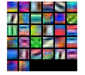
(Epoch 1 / 1) train acc: 0.476000; val_acc: 0.470000

5.13 cell18 可视化训练的特征

代码作业已经提供，有兴趣的读者可以阅读怎么可视化的代码。

下面是结果：

5.14 cell19 Spatial Batch Normalization

前面我们实现了Batch Normalization。但是怎么把它用到卷积层呢？对于全连接层，我们对每一个激活函数的输入单独进行batch normalization。对于卷积层，它的输入是C × H × W 的图像，我们需要对一个Channel的图像进行batch normalization。

5.14.1 forward

def spatial_batchnorm_forward(x, gamma, beta, bn_param):

  Inputs:
  - x: 输入数据shape (N, C, H, W)
  - gamma: scale参数 shape (C,)
  - beta: 平移参数 shape (C,)
  - bn_param: Dictionary包括:
    - mode: 'train' 或者 'test'; 必须有的
    - eps: 保持数值计算稳定的一个很小的常量
    - momentum: 计算running mean/variance的常量，前面也讲过。   
      如果momentum=0 那么每次都丢弃原来的值，只用当前最新值。
      momentum=1 表示只用原来的值。默认0.9，大部分情况下不用修改
    - running_mean: 数组 shape (D,) 保存当前的均值
    - running_var 数组 shape (D,) 保存当前的方差

  Returns a tuple of:
  - out: 输出数据 shape (N, C, H, W)
  - cache: 用于backward的cache
  """
  out, cache = None, None

  #############################################################################
  # TODO: Implement the forward pass for spatial batch normalization.         #
  #                                                                           #
  # HINT: You can implement spatial batch normalization using the vanilla     #
  # version of batch normalization defined above. Your implementation should  #
  # be very short; ours is less than five lines.                              #
  #############################################################################
  N, C, H, W = x.shape
  temp_output, cache = batchnorm_forward(x.transpose(0,2,3,1).reshape((N*H*W,C)), gamma, beta, bn_param)
  out = temp_output.reshape(N,H,W,C).transpose(0,3,1,2)

  #############################################################################
  #                             END OF YOUR CODE                              #
  #############################################################################

  return out, cache

代码这样3行：

1. 通过x.shape获得输入的N, C, H, W代表batchSize，Channel数，Height和Width
2. 把(N, C, H, W)的4维tensor变成(N H W,C)的2维tensor。因为要把第二维C放到最后，所以首先transponse(0,2,3,1)把第二维放到第四维，然后原来的第三和四维分别变成第二和三维。然后在reshape成二维的(N H W, C)。这样就直接调用之前的batchnorm_forward。
   transpose(0,2,3,1)的意思就是：把原来的第0维放到新的第0维【 不变】，把原来的第2维放到现在的第1维，把原来的第3维放到现在的第2维，把原来的第1维放到第3维。【主要这一段我说的时候下标是从0开始的了】
3. 计算完成后我们需要把它恢复成(N, C, H, W)的4维tensor

运行这cell进行测试：

Before spatial batch normalization:
  Shape:  (2, 3, 4, 5)
  Means:  [ 10.55377221  10.73790598   9.53943534]
  Stds:  [ 3.78632253  3.62325432  3.74675181]
After spatial batch normalization:
  Shape:  (2, 3, 4, 5)
  Means:  [  5.66213743e-16  -1.38777878e-16   7.43849426e-16]
  Stds:  [ 0.99999965  0.99999962  0.99999964]
After spatial batch normalization (nontrivial gamma, beta):
  Shape:  (2, 3, 4, 5)
  Means:  [ 6.  7.  8.]
  Stds:  [ 2.99999895  3.99999848  4.99999822]

5.14.2 backward

和forward很类似

  N,C,H,W = dout.shape
  dx_temp, dgamma, dbeta = batchnorm_backward_alt(dout.transpose(0,2,3,1).reshape((N*H*W,C)),cache)
  dx = dx_temp.reshape(N,H,W,C).transpose(0,3,1,2)

下面是gradient check的结果：

dx error:  1.24124210224e-07
dgamma error:  1.440787364e-12
dbeta error:  1.19492399319e-11

5.15 实现一个validation数据上准确率超过65%的网络

这其实是一个开放的问题，这是一个很不错的问题。cifar10相对于mnist，分类数不变，但是分类难度要大不少。我们之前随便用一个3层的全连接网络就能实现95%以上的准确率，但是cifar10要实现这么高的准确率就不容易了。另一方面，相对于imagenet百万的训练数据，cifar的训练数据量只有50000，即使用十几层的卷积网络，在笔记本上训练几个小时也就收敛了。而训练imagenet即使用GPU也需要好几天才能收敛。所以用这个数据集来练手是个不错的选择。目前ResNet和Inception v4【不懂的读者不要着急，后面我们会简单的介绍它的思想，自己实现这种网络也不难】在这个数据上都能到95%以上的准确率。作业让我们达到65%的要求不算很高，读者可以尝试不同的网络层数，不同的dropout和learning_rate。

下面是我的一些调参经验：

1. learning_rate非常重要，刚开始要大，之后用lr_decay让它变小。如果发现开始loss下降很慢，那么可以调大这个参数。如果loss时而变大时而变小【当然偶尔反复是正常的】，那么可能是learning_rate过大了。
2. 最原始的sgd效果不好，最好用adam或者rmsprop再加上momentum
3. 如果训练准确率和验证准确率差距过大，说明模型过拟合了，可以增大L2正则化参数reg，另外使用dropout也是可以缓解过拟合的。
4. batch norm非常有用，尽量使用
5. 越深的网络效果越好，当然要求的参数也越多，计算也越慢。后面我们会介绍一些使得我们可以训练更深网络的方法，比如著名的152层的ResNet以及参数很少的Inception系列算法，这些方法是最近一两年在ImageNet上名列前茅。

我这里就介绍VGG网络结构，原文为 Very Deep Convolutional Networks for Large-Scale Image Recognition 。这种网络结构很简单，LSVRC14的比赛上取得了很好的成绩。这一年另外一个比较好的是GoogLeNet，也就是inception v1。LSVRC15上的冠军就是ResNet，之后inception发展到v2/3(v2和v3其实是一篇论文出来的)和v4。这基本就是Image Classification比较state of the art的一些方法了。后面我们会简单的介绍ResNet和Inception的基本思想，这里我们先介绍VGG和它的实现方法。

1. VGG简介

VGG其实也没有什么的新东西，就是使用3 × 3的卷积和pooling实现比较深(16-19)层【当然ResNet出来后就不敢说自己深了】的网络结构。
VGG的结构如下图：

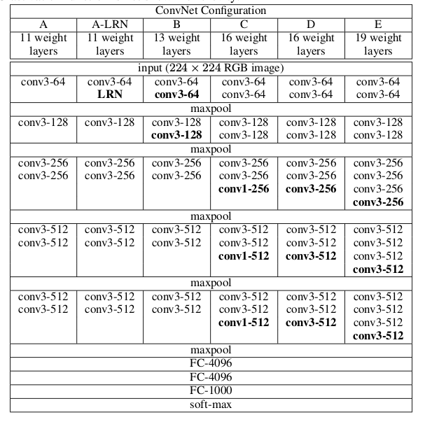
它的特点是：

所有的卷积都是 3×3，padding是1，stride是1，这样保证卷积后图像的大小不变，把几个filter数量一样的几个conv-relu合成一组，最后再用pooling把图像大小减半，图像大小减半之后一般就会增加filter的数量。最后接几个全连接层，最后一层是softmax。

我这里用我们已有的基础代码简单的实现了一个支持batch normalization和dropout的VGG，代码细节就不赘述了，有兴趣的读者可以参考代码。

class VGGlikeConvNet(object):
  """
  A flexible convolutional network with the following architecture:
  [(CONV-SBN-RELU)*A-POOL]*B - (FC-BN-RELU)*K - SOFTMAX

  The network operates on minibatches of data that have shape (N, C, H, W)
  consisting of N images, each with height H and width W and with C input
  channels.
  """
  def __init__(self, input_dim=(3, 32, 32), num_filters=[64, 128, 256, 512, 512], filter_size=3,
                       hidden_dims=[1024, 1024], num_classes=10, weight_scale=1e-2, reg=1e-3,
                       As=[2,2,3,3,3],use_batchnorm=True,
                       dropout=0, dtype=np.float32, seed=None):

    """
    Inputs:
    - input_dim: Tuple (C, H, W) giving size of input data
    - num_filters: A list of integers giving the filters to use in each "MAIN" convolutional layer
    - filter_size: Size of filters to use in the convolutional layer
    - hidden_dim: A list of integers giving the size of each hidden layer.
    - num_classes: Number of scores to produce from the final affine layer.
    - weight_scale: Scalar giving standard deviation for random initialization
      of weights.
    - reg: Scalar giving L2 regularization strength
    - As: Numbers of "SUB" convolution-layer replications in each num_filter
    - dtype: numpy datatype to use for computation.
    """
    self.params = {}
    self.reg = reg
    self.dtype = dtype
    self.use_dropout = dropout > 0
    self.use_batchnorm = use_batchnorm
    self.filter_size=filter_size
    self.hidden_dims=hidden_dims
    C, H, W = input_dim
    self.num_filters=num_filters
    self.As=As

    # With batch normalization we need to keep track of running means and
    # variances, so we need to pass a special bn_param object to each batch
    # normalization layer. You should pass self.bn_params[0] to the forward pass
    # of the first batch normalization layer, self.bn_params[1] to the forward
    # pass of the second batch normalization layer, etc.
    self.bn_params = {}

    for i in range(1, len(num_filters)+1):
      num_filter=num_filters[i-1]

      for j in range(1, As[i-1]+1):
        #debug
        ss=str(i)+","+str(j)
        print (H,W,C, num_filter,  filter_size, filter_size)
        self.params['W' + ss] = np.random.normal(0, weight_scale,
                                                                (num_filter, C, filter_size, filter_size))
        self.params['b' + ss] = np.zeros(num_filter)

        C=num_filter
        if self.use_batchnorm:
          self.params['beta' + ss] = np.zeros(num_filter)
          self.params['gamma'+ ss]=np.ones(num_filter)
          self.bn_params[ss]={'mode': 'train'}
      #max-pooling size/=2
      H/=2
      W/=2

    # full connected layers
    for i in range(1, len(hidden_dims)+1):
      layer_input_dim = C*H*W if i == 1 else hidden_dims[i - 2]
      layer_output_dim = hidden_dims[i - 1]
      print (layer_input_dim, layer_output_dim)
      self.params['W' + str(i)] = np.random.normal(0, weight_scale, (layer_input_dim, layer_output_dim))

      self.params['b' + str(i)] = np.zeros(layer_output_dim)

      if self.use_batchnorm:
        self.params['beta' + str(i)] = np.zeros(layer_output_dim)
        self.params['gamma' + str(i)] = np.ones(layer_output_dim)
        self.bn_params[str(i)]={'mode': 'train'}
    # softmax layer
    softmax_input_dim=hidden_dims[-1]
    softmax_output_dim=num_classes
    print (softmax_input_dim, softmax_output_dim)
    self.params['W_softmax'] = np.random.normal(0, weight_scale, (softmax_input_dim, softmax_output_dim))
    self.params['b_softmax'] = np.zeros(softmax_output_dim)
    self.dropout_param = {}
    if self.use_dropout:
      self.dropout_param = {'mode': 'train', 'p': dropout}
      if seed is not None:
        self.dropout_param['seed'] = seed


    # Cast all parameters to the correct datatype
    for k, v in self.params.iteritems():
      self.params[k] = v.astype(dtype)

  def loss(self, X, y=None):
    """
    Compute loss and gradient for the fully-connected net.

    Input / output: Same as TwoLayerNet above.
    """
    X = X.astype(self.dtype)
    mode = 'test' if y is None else 'train'

    # Set train/test mode for batchnorm params and dropout param since they
    # behave differently during training and testing.
    if self.dropout_param is not None:
      self.dropout_param['mode'] = mode
    if self.use_batchnorm:
      for bn_param in self.bn_params:
        self.bn_params[bn_param]['mode'] = mode

    scores = None

    conv_caches={}
    relu_caches={}
    bn_caches={}
    affine_relu_caches={}
    affine_bn_relu_caches={}
    dropout_caches={}
    pool_caches={}
    conv_param = {'stride': 1, 'pad': (self.filter_size - 1) / 2}

    # pass pool_param to the forward pass for the max-pooling layer
    pool_param = {'pool_height': 2, 'pool_width': 2, 'stride': 2}
    current_input = X

    # conv layers
    for i in range(1, len(self.num_filters)+1):
      for j in range(1, self.As[i-1]+1):
        ss=str(i) + "," +str(j)
        keyW = 'W' + ss
        keyb = 'b' + ss
        if not self.use_batchnorm:
          conv_out, conv_cache = conv_forward_fast(current_input, self.params[keyW], self.params[keyb], conv_param)
          relu_out, relu_cache = relu_forward(conv_out)
          conv_caches[ss]=conv_cache
          relu_caches[ss]=relu_cache
          current_input=relu_out
        else:
          key_gamma = 'gamma' + ss
          key_beta = 'beta' + ss
          conv_out, conv_cache = conv_forward_fast(current_input, self.params[keyW], self.params[keyb], conv_param)
          bn_out, bn_cache=spatial_batchnorm_forward(conv_out, self.params[key_gamma], self.params[key_beta], self.bn_params[ss])
          relu_out, relu_cache = relu_forward(bn_out)
          conv_caches[ss] = conv_cache
          relu_caches[ss] = relu_cache
          bn_caches[ss] = bn_cache
          current_input = relu_out
      pool_out, pool_cache = max_pool_forward_fast(current_input, pool_param)
      pool_caches[str(i)]=pool_cache
      current_input=pool_out

    # full connected layers
    for i in range(1, len(self.hidden_dims) + 1):
      keyW = 'W' + str(i)
      keyb = 'b' + str(i)

      if not self.use_batchnorm:
        current_input, affine_relu_caches[i] = affine_relu_forward(current_input, self.params[keyW], self.params[keyb])

      else:
        key_gamma = 'gamma' + str(i)
        key_beta = 'beta' + str(i)
        current_input, affine_bn_relu_caches[i] = affine_bn_relu_forward(current_input, self.params[keyW],
                                                                        self.params[keyb],
                                                                        self.params[key_gamma], self.params[key_beta],
                                                                        self.bn_params[str(i)])

      if self.use_dropout:
        current_input, dropout_caches[i] = dropout_forward(current_input, self.dropout_param)


    # softmax
    keyW = 'W_softmax'
    keyb = 'b_softmax'
    affine_out, affine_cache = affine_forward(current_input, self.params[keyW], self.params[keyb])

    scores=affine_out


    # If test mode return early
    if mode == 'test':
      return scores

    loss, grads = 0.0, {}

    loss, dscores = softmax_loss(scores, y)

    # last layer:
    affine_dx, affine_dw, affine_db = affine_backward(dscores, affine_cache)

    grads['W_softmax'] = affine_dw + self.reg * self.params['W_softmax']
    grads['b_softmax'] = affine_db

    loss += 0.5 * self.reg * (np.sum(self.params['W_softmax'] * self.params['W_softmax']))

    # full connected layers
    for i in range(len(self.hidden_dims), 0, -1):
      if self.use_dropout:
        affine_dx = dropout_backward(affine_dx, dropout_caches[i])

      if not self.use_batchnorm:
        affine_dx, affine_dw, affine_db = affine_relu_backward(affine_dx, affine_relu_caches[i])
      else:
        affine_dx, affine_dw, affine_db, dgamma, dbeta = affine_bn_relu_backward(affine_dx, affine_bn_relu_caches[i])
        grads['beta' + str(i)] = dbeta
        grads['gamma' + str(i)] = dgamma

      keyW = 'W' + str(i)
      keyb = 'b' + str(i)
      loss += 0.5 * self.reg * (np.sum(self.params[keyW] * self.params[keyW]))
      grads[keyW] = affine_dw + self.reg * self.params[keyW]

      grads[keyb] = affine_db

    # conv layers
    conv_dx=affine_dx
    for i in range(len(self.num_filters), 0, -1):
      dpool_out=conv_dx
      conv_dx=max_pool_backward_fast(dpool_out, pool_caches[str(i)])

      for j in range(self.As[i-1],0,-1):
        ss=str(i) + "," +str(j)
        keyW = 'W' + ss
        keyb = 'b' + ss
        if not self.use_batchnorm:
          drelu_out=conv_dx
          relu_cache=relu_caches[ss]
          conv_cache=conv_caches[ss]
          dconv_out=relu_backward(drelu_out, relu_cache)
          conv_dx, conv_dw, conv_db=conv_backward_fast(dconv_out, conv_cache)

          loss += 0.5 * self.reg * (np.sum(self.params[keyW] * self.params[keyW]))
          grads[keyW] = conv_dw + self.reg * self.params[keyW]
          grads[keyb] = conv_db

        else:
          key_gamma = 'gamma' + ss
          key_beta = 'beta' + ss

          drelu_out = conv_dx
          relu_cache = relu_caches[ss]
          conv_cache = conv_caches[ss]
          bn_cache=bn_caches[ss]

          dbn_out = relu_backward(drelu_out, relu_cache)
          dconv_out, dgamma, dbeta=spatial_batchnorm_backward(dbn_out, bn_cache)
          grads[key_beta] = dbeta
          grads[key_gamma] = dgamma

          conv_dx, conv_dw, conv_db = conv_backward_fast(dconv_out, conv_cache)

          loss += 0.5 * self.reg * (np.sum(self.params[keyW] * self.params[keyW]))
          grads[keyW] = conv_dw + self.reg * self.params[keyW]
          grads[keyb] = conv_db

    ############################################################################
    #                             END OF YOUR CODE                             #
    ############################################################################

    return loss, grads

2. 使用VGG完成作业

我没有使用太深的VGG，因为是在笔记本上跑，参数也没有仔细调过，跑了一下可以得到85%以上的准确率，有兴趣的读者可以自己调调网络层数和超参数，应该是有可能得到90%以上准确率的

model = VGGlikeConvNet(input_dim=(3, 32, 32), num_filters=[64, 64, 128, 256], filter_size=3,
                       hidden_dims=[64, 64], num_classes=10, weight_scale=1e-2, reg=1e-3, As=[2,2,3,3],
                       dropout=0.2,
                       dtype=np.float32)

solver=Solver(model, data,
       num_epochs=10, batch_size=50,
       update_rule='adam',
       lr_decay=0.95,
       optim_config={'learning_rate': 5e-4},
       verbose=True, print_every=20) 

solver.train()

下面是结果：

(Iteration 9741 / 9800) loss: 0.733453
(Iteration 9761 / 9800) loss: 0.645659
(Iteration 9781 / 9800) loss: 0.564387
(Epoch 10 / 10) train acc: 0.927000; val_acc: 0.854000

本篇文章就到这里，在下一篇文章中，我将使用caffe在imagnet上训练AlexNet以及使用训练好的模型进行分类，敬请关注。

---