sklearn集成方法
集成方法
集成方法是训练很多基学习器,然后用这些基学习器去对进行分类或者回归,最后取所有结果中比例最大的作为模型的结果
投票分类器(Voting Classifiers)
- 定义:对于一个训练集,有很多分类器,比如说Logistic、KNN、SVM等。对于一个样本,我们给出所有分类器的分类结果,然后利用这个结果对样本的分类进行预测
- hard voting classifier :不考虑分类器的差别,比如说他们的准确性等,直接取投票数最多的类别,将其作为我们最后的对于该样本的分类结果
- soft voting classifier:利用所有分类器给出的各个类别的概率,最后利用各个类别的概率之和进行预测,doft voting的准确率要略微高于hard voting,因为它考虑了每个模型的不同
- 在很多情况下,投票分类器的精度会比集合里最好的分类器的精度还要高(对于大多数测试集),因为这种集成方法提高了模型的鲁棒性。
- 当集成方法中的基学习器之间互相独立时,集成方法的效果会更好
from sklearn.ensemble import RandomForestClassifier
from sklearn.ensemble import VotingClassifier
from sklearn.linear_model import LogisticRegression
from sklearn.svm import SVC
from sklearn.model_selection import train_test_split
from sklearn.datasets import make_moons
from sklearn.metrics import accuracy_score

# 导入数据
X, y = make_moons(n_samples=500, noise=0.30, random_state=42)
X_train, X_test, y_train, y_test = train_test_split(X, y, random_state=42)

# 三个基学习器
log_clf = LogisticRegression()
rf_clf = RandomForestClassifier()
svm_clf = SVC()
# 投票分类器
voting_clf = VotingClassifier( estimators=[("lr", log_clf), ("rf", rf_clf), ("svc", svm_clf)], voting="hard" )
# voting_clf.fit( X_train, y_train )

for clf in ( log_clf, rf_clf, svm_clf, voting_clf ):
    clf.fit( X_train, y_train )
    y_pred = clf.predict( X_test )
    print( clf.__class__.__name__, accuracy_score(y_test, y_pred) )
LogisticRegression 0.864
RandomForestClassifier 0.88
SVC 0.888
VotingClassifier 0.896
Bagging和Boosting
- 怎样得到很多基学习器:可以选择很多不同的训练算法,也可以对于每个基学习器,都选择相同的训练算法,但是对于每个基学习器,都用不同的子数据集或者子特征集进行训练
- 有放回抽样:即数据集允许重复(对于每一个基学习器),这也叫bagging
- 无放回抽样:即数据不允许重复,这也叫pasting
both bagging and pasting allow training instances to be sampled several times across multiple predictors, but only bagging allows training instances to be sampled several times for the same predictor
- 得到很多基学习器之后,就可以利用统计的方法进行分类或者回归
- sklearn中的BaggingClassifier可以实现Bagging
- n_estimators:基学习器的数量
- max_samples:每个基学习器中的样本数,如果是整形,则就是样本个数;如果是float,则是样本个数占所有训练集样本个数的比例
- bootstrap :是否采用有放回抽样(bagging),为True表示采用,否则为pasting。默认为True
- n_jobs:并行运行的作业数量。-1时,个数为处理器核的个数
- oob_socre:为True时,对模型进行out-of-bag的验证,即在一个基学习器中,没有用于训练的数据用于验证
- 相对于单个的决策树,Bagging方法得到的分类边界更加平滑
- 相对于pasting方法来说,bagging方法中模型的偏差会偏大一点,因为它是采用有放回的抽样,所有模型中用到的数据的均匀性会差一点;但是因为这样,模型之间相对独立一点,因此bagging的方差会小一点。在实际使用过程中,bagging的效果一般会更好,因此一般使用bagging。但是对于具体的问题,我们也可以用交叉验证验证两种模型的性能。
- Out-of-bag Evaluation:每个模型中只会使用到一部分的数据集,因此剩下的数据集(没有用在)可以用于对模型进行验证
- Bagging也支持对特征的采样,可以用
max_features和bootstrap_features参数进行设置,这在处理高位特征输入的训练数据中十分有效,可以降低模型的复杂度以及过拟合的风险。同时对样本和特征进行采样称为Random Patches Method,保留所有的样本,只对特征进行采样称为Random Subspaces method
from sklearn.ensemble import BaggingClassifier
from sklearn.tree import DecisionTreeClassifier

bag_clf = BaggingClassifier( DecisionTreeClassifier(), n_estimators=500, max_samples=100, bootstrap=True, n_jobs=-1 )

bag_clf.fit( X_train, y_train )
y_pred = bag_clf.predict( X_test )
pred_score = accuracy_score( y_pred, y_test )
print( pred_score )
0.912
%matplotlib inline
import matplotlib.pyplot as plt
from matplotlib.colors import ListedColormap
from sklearn.tree import DecisionTreeClassifier
import numpy as np

def plot_decision_boundary(clf, X, y, axes=[-1.5, 2.5, -1, 1.5], alpha=0.5, contour=True):
    x1s = np.linspace(axes[0], axes[1], 100)
    x2s = np.linspace(axes[2], axes[3], 100)
    x1, x2 = np.meshgrid(x1s, x2s)
    X_new = np.c_[x1.ravel(), x2.ravel()]
    y_pred = clf.predict(X_new).reshape(x1.shape)
    custom_cmap = ListedColormap(['#fafab0','#9898ff','#a0faa0'])
    plt.contourf(x1, x2, y_pred, alpha=0.3, cmap=custom_cmap, linewidth=10)
    if contour:
        custom_cmap2 = ListedColormap(['#7d7d58','#4c4c7f','#507d50'])
        plt.contour(x1, x2, y_pred, cmap=custom_cmap2, alpha=0.8)
    plt.plot(X[:, 0][y==0], X[:, 1][y==0], "yo", alpha=alpha)
    plt.plot(X[:, 0][y==1], X[:, 1][y==1], "bs", alpha=alpha)
    plt.axis(axes)
    plt.xlabel(r"$x_1$", fontsize=18)
    plt.ylabel(r"$x_2$", fontsize=18, rotation=0)
    return

tree_clf = DecisionTreeClassifier(random_state=42)
tree_clf.fit(X_train, y_train)
y_pred_tree = tree_clf.predict(X_test)

plt.figure(figsize=(8,3))
plt.subplot(121)
plot_decision_boundary(tree_clf, X, y)
plt.title("Decision Tree", fontsize=14)
plt.subplot(122)
plot_decision_boundary(bag_clf, X, y)
plt.title("Decision Trees with Bagging", fontsize=14)
plt.show()
bag_clf = BaggingClassifier( DecisionTreeClassifier(), n_estimators=500, max_samples=100, bootstrap=True, n_jobs=-1, oob_score=True )
bag_clf.fit( X_train, y_train )
print( bag_clf.oob_score_ )
y_pred = bag_clf.predict( X_test )
print( accuracy_score(y_test, y_pred) )
# 输出bagging的概率矩阵
df = bag_clf.oob_decision_function_
# print( df )
0.896
0.896
随机森林(Random Forests)
- 随机森林一般是用bagging方法进行训练,每个决策树中使用的样本数都是全部的训练集,RandomForestClassifier中的参数与决策树基本一致,都是对决策树的形状等性质做一些规定
- 相比于Bagging方法,随机森林引入了一些额外的随机性,因为它不是在所有的特征中选择最好的分类特征用于分离一个节点,而是在随机的一些特征中选择最优的节点分割方法。这会增大模型的偏差,但是减小了模型的方差。
- 如果在bagging方法中设置模型随机选择特征进行基学习器的训练,那么它与随机森林等价(其他参数相同的情况下)
Extra-Trees
- 随机森林中,每个决策树的特征是随机的;而如果在每次选择分割节点的对应特征的阈值时,选择随机的阈值进行分割,而非之前决策树中使用的最优的方法,这会进一步增加模型的偏差,同时降低模型的方差。这种方法的训练速度也比之前的方法要更快
特征的重要性
- RF是white bx的模型,它的特征对模型的影响是可解释的,对于单个的决策树来说,越靠近根节点对应的特征越重要,而靠近叶子节点的特征的重要性相对小一些
from sklearn.ensemble import RandomForestClassifier
from sklearn.ensemble import ExtraTreesClassifier

rf_clf = RandomForestClassifier( n_estimators=500, max_leaf_nodes=16, n_jobs=-1 )
rf_clf.fit( X_train, y_train )
y_pred_clf = rf_clf.predict( X_test )
print( accuracy_score( y_pred_clf, y_test ) )

extra_tree_clf = ExtraTreesClassifier(n_estimators=500, max_leaf_nodes=16, n_jobs=-1)
extra_tree_clf.fit( X_train, y_train )
y_pred_clf = extra_tree_clf.predict( X_test )
print( accuracy_score( y_pred_clf, y_test ) )
0.928
0.912
from sklearn.datasets import load_iris

iris = load_iris()
rf_clf = RandomForestClassifier( n_estimators=500, n_jobs=-1 )
rf_clf.fit( iris.data, iris.target )
# rf_clf.feature_importances_中已经按照样本中特征的顺序进行了排序,与特征一一顺序对应
for name, score in zip( iris.feature_names, rf_clf.feature_importances_ ):
    print( name, score )
sepal length (cm) 0.103714253389
sepal width (cm) 0.0229312213868
petal length (cm) 0.435857047862
petal width (cm) 0.437497477363
import matplotlib
from sklearn.datasets import fetch_mldata
mnist = fetch_mldata('MNIST original')

rf_clf = RandomForestClassifier(random_state=42)
rf_clf.fit(mnist["data"], mnist["target"])

def plot_digit(data):
    image = data.reshape(28, 28)
    plt.imshow(image, cmap = matplotlib.cm.hot,
               interpolation="nearest")
    plt.axis("off")
    return

plot_digit(rf_clf.feature_importances_)
cbar = plt.colorbar(ticks=[rf_clf.feature_importances_.min(), rf_clf.feature_importances_.max()])
cbar.ax.set_yticklabels(['Not important', 'Very important'])
plt.show()
Boosting
- Boosting最初被称为hypothesis boosting,它指的是将若干弱学习器组合在一起,形成一个强学习器
- 基本思想是按次序训练学习器,并且修正之前的学习器
- 目前最常用的Boosting方法是AdaBoost和Gradient Boosting
AdaBoost
- AdaBoost也是有很多个基学习器,但是其基本思想是:每个基学习器的训练样本都会受到之前一个基学习器的影响,即在之前的基学习器中,那些被误分类的训练样本在下此次样本的选择中,会被赋予更大的比重,即学习器更关注之前的误分类样本
公式推导
参考链接:http://blog.csdn.net/GYQJN/article/details/45501185
对于二分类器来说,输入为训练集$T=\{(x_{1},y_{1}),(x_{2},y_{2}), ...(x_{N},y_{N})\}$。其中$x_{i}\in X \subseteq R^n ,y_{i}\in Y=\{-1,+1\}$
输出为最终分类器 G(x)
- 初始化训练数据的权值分布
D1=(w11,...,w1i,...,w1N),w1i=1N,i=1,2,...,N
在初始的时候,分类器对于各个样本的权值是相等的 对于m=1,2,3,…M(M为AdaBoost包含的基学习器个数)
- 使用具有权值分布 Dm 的训练数据集学习,得到基本分类器
Gm:X→{−1,+1} - 计算 Gm(x) 在训练集上的分类误差率
em=P(Gm(xi)≠yi)=∑i=1nwmiI(Gm(xi)≠yi)
这里, I(Gm(xi)≠yi) 是示性函数,括号中的不等式成立时,值为1,否则为0 - 计算 Gm(x) 的系数
αm=12log1−emem
因此 αm 是关于 em 的递减函数,错误率更小的基学习器会对最终的分类器有更大的贡献 - 更新训练数据集的权值分布
Dm+1=(wm+1,1,...,wm+1,i,...,wm+1,N)
wm+1,i=wmiZmexp(−αmyiGm(xi))i=1,2,...,N
其中, Zm 是规划因子
Zm=∑i=1Nwmiexp(−αmyiGm(xi))
即所有的 wm,i 关于i相加结果为1 构建基本分类器的线性组合,得到最终的分类器
G(x)=sign(f(x))=sign(∑m=1MαmGm(x))由于AdaBoost在每次训练时,都需要用到之前的基学习器,因此无法实现多个基学习器共同训练的并行化
- 使用具有权值分布 Dm 的训练数据集学习,得到基本分类器
from sklearn.ensemble import AdaBoostClassifier

ada_clf = AdaBoostClassifier(
    DecisionTreeClassifier(max_depth=1), n_estimators=200,
    algorithm="SAMME.R", learning_rate=0.5, random_state=42)
ada_clf.fit(X_train, y_train)
plt.figure(figsize=(4,3))
plot_decision_boundary( ada_clf, X, y )
plt.show()
# AdaBoost的基本思想示例
m = len(X_train)

plt.figure(figsize=(8, 3))
for subplot, learning_rate in ((121, 1), (122, 0.5)):
    sample_weights = np.ones(m)
    for i in range(5):
        plt.subplot(subplot)
        svm_clf = SVC(kernel="rbf", C=0.05, random_state=42)
        svm_clf.fit(X_train, y_train, sample_weight=sample_weights)
        y_pred = svm_clf.predict(X_train)
        sample_weights[y_pred != y_train] *= (1 + learning_rate)
        plot_decision_boundary(svm_clf, X, y, alpha=0.2)
        plt.title("learning_rate = {}".format(learning_rate), fontsize=16)

plt.subplot(121)
plt.text(-0.7, -0.65, "1", fontsize=14)
plt.text(-0.6, -0.10, "2", fontsize=14)
plt.text(-0.5,  0.10, "3", fontsize=14)
plt.text(-0.4,  0.55, "4", fontsize=14)
plt.text(-0.3,  0.90, "5", fontsize=14)
plt.show()
Gradient Boosting
- GB与AdaBoost类似,也是依次在集成方法增加学习器,但是不同的是,AdaBoost是在每次迭代过程中调节训练数据的权重,而GB是在每次迭代过程中,采用之前的基学习器的残差来训练得到新的基学习器
- Gradient Boosted Regression Trees也叫GBRT
- sklearn中集成了GBRT,里面有一个学习率的超参数。如果这个参数设置的比较小,则需要更多的树来拟合训练集,但是预测效果一般会更好。
- 对于相同的GBRT,树的个数太多,容易造成过拟合现象
# GBRT的基本实现
from sklearn.tree import DecisionTreeRegressor
np.random.seed(42)
X = np.random.rand(100, 1) - 0.5
y = 3*X[:, 0]**2 + 0.05 * np.random.randn(100)

def plot_predictions(regressors, X, y, axes, label=None, style="r-", data_style="b.", data_label=None):
    x1 = np.linspace(axes[0], axes[1], 500)
    y_pred = sum(regressor.predict(x1.reshape(-1, 1)) for regressor in regressors)
    plt.plot(X[:, 0], y, data_style, label=data_label)
    plt.plot(x1, y_pred, style, linewidth=2, label=label)
    if label or data_label:
        plt.legend(loc="upper center", fontsize=16)
    plt.axis(axes)
    return

tree_reg1 = DecisionTreeRegressor( max_depth=2 )
tree_reg1.fit( X, y )
y2 = y - tree_reg1.predict( X )
tree_reg2 = DecisionTreeRegressor( max_depth=2 )
tree_reg2.fit( X, y2 )
y3 = y2 - tree_reg2.predict(X)
tree_reg3 = DecisionTreeRegressor(max_depth=2)
tree_reg3.fit(X, y3)
# t_pred = sum( tree.predict(X_new) for tree in ( tree_reg1, tree_reg2, tree_reg3 )  )

plt.figure(figsize=(9,9))
plt.subplot(321)
plot_predictions([tree_reg1], X, y, axes=[-0.5, 0.5, -0.1, 0.8], label="$h_1(x_1)$", style="g-", data_label="Training set")
plt.ylabel("$y$", fontsize=12, rotation=0)
plt.title("Residuals and tree predictions", fontsize=12)

plt.subplot(322)
plot_predictions([tree_reg1], X, y, axes=[-0.5, 0.5, -0.1, 0.8], label="$h(x_1) = h_1(x_1)$", data_label="Training set")
plt.ylabel("$y$", fontsize=12, rotation=0)
plt.title("Ensemble predictions", fontsize=12)

plt.subplot(323)
plot_predictions([tree_reg2], X, y2, axes=[-0.5, 0.5, -0.5, 0.5], label="$h_2(x_1)$", style="g-", data_style="k+", data_label="Residuals")
plt.ylabel("$y - h_1(x_1)$", fontsize=12)

plt.subplot(324)
plot_predictions([tree_reg1, tree_reg2], X, y, axes=[-0.5, 0.5, -0.1, 0.8], label="$h(x_1) = h_1(x_1) + h_2(x_1)$")
plt.ylabel("$y$", fontsize=12, rotation=0)

plt.subplot(325)
plot_predictions([tree_reg3], X, y3, axes=[-0.5, 0.5, -0.5, 0.5], label="$h_3(x_1)$", style="g-", data_style="k+")
plt.ylabel("$y - h_1(x_1) - h_2(x_1)$", fontsize=16)
plt.xlabel("$x_1$", fontsize=12)

plt.subplot(326)
plot_predictions([tree_reg1, tree_reg2, tree_reg3], X, y, axes=[-0.5, 0.5, -0.1, 0.8], label="$h(x_1) = h_1(x_1) + h_2(x_1) + h_3(x_1)$")
plt.xlabel("$x_1$", fontsize=12)
plt.ylabel("$y$", fontsize=12, rotation=0)
plt.show()
# sklearn中集成了GBRT
from sklearn.ensemble import GradientBoostingRegressor

gbrt = GradientBoostingRegressor( max_depth=2, n_estimators=3, learning_rate=1.0 )
gbrt.fit( X, y )
plt.figure( figsize=(8,3) )
plt.subplot(121)
plot_predictions( [gbrt], X, y, axes=[-0.5, 0.5, -0.1, 0.8], label="$n\_estimators=3$" )

gbrt = GradientBoostingRegressor( max_depth=2, n_estimators=30, learning_rate=1.0 )
plt.subplot( 122 )
gbrt.fit( X, y )
plot_predictions( [gbrt], X, y, axes=[-0.5, 0.5, -0.1, 0.8], label="$n\_estimators=200$" )
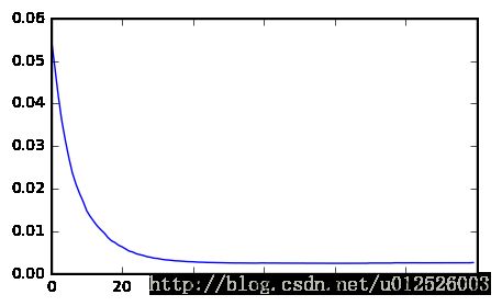
- 为了防止过拟合,可以采用
early stopping的方法。先设置一个较大的树的个数,然后从这里面找出MSE最小的一棵树,这棵树所在的下标就是我们最终需要的树的个数 - GBRT中也包含
subsample的超参数,相当于在训练一棵树的时候,只采用这么多的训练样本,类似于随机梯度下降的方法。
from sklearn.model_selection import train_test_split
from sklearn.metrics import mean_squared_error

X_train, X_val, y_train, y_val = train_test_split( X, y )

gbrt = GradientBoostingRegressor(max_depth=2, n_estimators=120)
gbrt.fit( X_train, y_train )

errors = [ mean_squared_error(y_val, y_pred) for y_pred in gbrt.staged_predict( X_val ) ]
best_n_estimators = np.argmin( errors )
print( "best number of estimators is : ", best_n_estimators )
plt.figure( figsize=(5,3) )
plt.plot( errors )
plt.show()

gbrt_best = GradientBoostingRegressor( max_depth=2, n_estimators=best_n_estimators )
gbrt_best.fit( X_train, y_train )
best number of estimators is : 84
GradientBoostingRegressor(alpha=0.9, criterion='friedman_mse', init=None,
             learning_rate=0.1, loss='ls', max_depth=2, max_features=None,
             max_leaf_nodes=None, min_impurity_decrease=0.0,
             min_impurity_split=None, min_samples_leaf=1,
             min_samples_split=2, min_weight_fraction_leaf=0.0,
             n_estimators=84, presort='auto', random_state=None,
             subsample=1.0, verbose=0, warm_start=False)
Stacking
- Stacking不是简单的对所有模型进行简单的平均或者加权聚合,而是训练出一个模型,来对这些基学习器进行聚合。
- Stacking首先训练出很多基学习器,然后再训练一个元学习器(meta learner或者blender),对这些基学习器进行聚合
- 训练方法:将训练集分为两个子集(subset)。其中一个子集用于训练所有的基学习器(假设有M个基学习器),用这些基学习对另一个子集的训练集(假设有N个样本)进行预测,得到NXM的预测结果,然后采用线性回归或者决策树等方法,将另一个子集的训练结果作为输入,将训练集的输出作为输出,进行训练,得到元学习器
- sklearn不直接支持stacking算法,但是可以自己封装一下