TensorFlow2——Keras训练和评估

 
TensorFlow 2.0中一般有两种情况下的训练、评估和预测（推断）模型：

1. 使用内置APIs进行训练和验证（例如model.fit(), model.evaluate(), model.predict())。
2. 使用紧急执行和GradientTape对象从头开始编写自定义循环。

一般来说，无论是使用内置循环还是编写自己的循环，模型训练和评估在各种Keras模型中的工作方式都是相同的——Sequential模型、使用函数API构建的模型以及通过模型子类化从头开始编写的模型。

 

1 、使用内置的训练和评估循环

将数据传递到模型的内置训练循环时，应该使用Numpy数组（如果数据很小并且适合内存），或者使用 tf.data Dataset 对象。

接下来，将使用MNIST数据集作为Numpy数组，以演示如何使用optimizers, losses, 和metrics。
 

API概述：第一个端到端示例

这里，使用函数API构建模型：

import tensorflow as tf
import numpy as np
from tensorflow import keras
from tensorflow.keras import layers

inputs = keras.Input(shape=(784,), name='digits')
x = layers.Dense(64, activation='relu', name='dense_1')(inputs)
x = layers.Dense(64, activation='relu', name='dense_2')(x)
outputs = layers.Dense(10, name='predictions')(x)

model = keras.Model(inputs=inputs, outputs=outputs)

典型的端到端工作流是这样的，包括训练、对原始训练数据生成的数据集的验证，以及对测试数据的最终评估：

1）加载数据集：

(x_train, y_train), (x_test, y_test) = keras.datasets.mnist.load_data()

# Preprocess the data (these are Numpy arrays)
x_train = x_train.reshape(60000, 784).astype('float32') / 255
x_test = x_test.reshape(10000, 784).astype('float32') / 255

y_train = y_train.astype('float32')
y_test = y_test.astype('float32')

# Reserve 10,000 samples for validation
x_val = x_train[-10000:]
y_val = y_train[-10000:]
x_train = x_train[:-10000]
y_train = y_train[:-10000]

2）指定训练配置（optimizer, loss, metrics）

model.compile(optimizer=keras.optimizers.RMSprop(),  # Optimizer
              # Loss function to minimize
              loss=keras.losses.SparseCategoricalCrossentropy(from_logits=True),
              # List of metrics to monitor
              metrics=['sparse_categorical_accuracy'])

3）通过将数据分为大小为“batch_size”的“batches”来训练模型，并在给定数量的“epochs”中重复遍历整个数据集

print('# Fit model on training data')
history = model.fit(x_train, y_train,
                    batch_size=64,
                    epochs=3,
                    # We pass some validation for
                    # monitoring validation loss and metrics
                    # at the end of each epoch
                    validation_data=(x_val, y_val))

print('\nhistory dict:', history.history)

返回的“history”对象保存训练期间loss值和metric值。

4）最后，使用测试集数据进行评估和预测：

# Evaluate the model on the test data using `evaluate`
print('\n# Evaluate on test data')
results = model.evaluate(x_test, y_test, batch_size=128)
print('test loss, test acc:', results)

# Generate predictions (probabilities -- the output of the last layer)
# on new data using `predict`
print('\n# Generate predictions for 3 samples')
predictions = model.predict(x_test[:3])
print('predictions shape:', predictions.shape)

 

loss、metrics和optimizer

要使用fit训练模型，需要指定loss函数、optimizer，还可以选择指定一些要监视的metrics。

将这些作为参数传递给模型的compile（）方法：

model.compile(optimizer=keras.optimizers.RMSprop(learning_rate=1e-3),
              loss=keras.losses.SparseCategoricalCrossentropy(from_logits=True),
              metrics=[keras.metrics.sparse_categorical_accuracy])

也可以通过字符串标识符的方式：

model.compile(optimizer='rmsprop',
              loss=keras.losses.SparseCategoricalCrossentropy(from_logits=True),
              metrics=['sparse_categorical_accuracy'])

其中，metrics参数是一个列表——模型可以有任意数量的metrics。
 

Keras API 中内置的optimizers、losses和metrics：

Optimizers:

SGD() (with or without momentum)
RMSprop()
Adam()
etc.

Losses:

MeanSquaredError()
KLDivergence()
CosineSimilarity()
etc.

Metrics:

AUC()
Precision()
Recall()
etc.

 

自定义 losses

有两种方法可以自定义losses。

方法一：创建一个函数，该函数的输入为 y_true 和 y_pred 。该函数计算实际数据和预测之间的平均绝对误差：

def basic_loss_function(y_true, y_pred):
    return tf.math.reduce_mean(tf.abs(y_true - y_pred))

model.compile(optimizer=keras.optimizers.Adam(),
              loss=basic_loss_function)

model.fit(x_train, y_train, batch_size=64, epochs=3)

如果需要一个loss函数，它需要除 y_true 和 y_pred 之外的参数，您可以子类化 tf.keras.losses.Loss类并实现以下两种方法：

	__init__(self)：接受在调用loss函数期间要传递的参数
	call(self, y_true, y_pred)：使用目标（y_true）和模型预测（y_pred）计算模型的损失

在计算损失时，可以在call（）期间使用传递到__init__()的参数。

方法二：实现计算BinaryCrossEntropy损失的WeightedCrossEntropy损失函数，其中某个类或整个函数的损失可以由标量修改。

class WeightedBinaryCrossEntropy(keras.losses.Loss):
    """
    Args:
      pos_weight: Scalar to affect the positive labels of the loss function.
      weight: Scalar to affect the entirety of the loss function.
      from_logits: Whether to compute loss from logits or the probability.
      reduction: Type of tf.keras.losses.Reduction to apply to loss.
      name: Name of the loss function.
    """
    def __init__(self, pos_weight, weight, from_logits=False,
                 reduction=keras.losses.Reduction.AUTO,
                 name='weighted_binary_crossentropy'):
        super().__init__(reduction=reduction, name=name)
        self.pos_weight = pos_weight
        self.weight = weight
        self.from_logits = from_logits

    def call(self, y_true, y_pred):
        ce = tf.losses.binary_crossentropy(
            y_true, y_pred, from_logits=self.from_logits)[:,None]
        ce = self.weight * (ce*(1-y_true) + self.pos_weight*ce*(y_true))
        return ce

one_hot_y_train = tf.one_hot(y_train.astype(np.int32), depth=10)

model.compile(
    optimizer=keras.optimizers.Adam(),
    loss=WeightedBinaryCrossEntropy(
        pos_weight=0.5, weight = 2, from_logits=True)
)
model.fit(x_train, one_hot_y_train, batch_size=64, epochs=5)

 

自定义metrics

可以通过子类化Metric类来轻松创建自定义metrics，并且需要实现4个方法：

	__init__(self)：创建状态变量。
	update_state(self, y_true, y_pred, sample_weight=None)：使用目标y_true和模型预测y_pred更新状态变量。
	result(self)：使用状态变量来计算最终结果。
	reset_states(self)：重新初始化度量的状态。

状态更新和结果计算是分开的，因为在某些情况下，结果计算大，并且只能定期进行。

下面是一个简单的示例，演示如何实现CategoricalTruePositives metric，计算正确分类为属于给定类的样本数：

class CategoricalTruePositives(keras.metrics.Metric):

    def __init__(self, name='categorical_true_positives', **kwargs):
      super(CategoricalTruePositives, self).__init__(name=name, **kwargs)
      self.true_positives = self.add_weight(name='tp', initializer='zeros')

    def update_state(self, y_true, y_pred, sample_weight=None):
      y_pred = tf.reshape(tf.argmax(y_pred, axis=1), shape=(-1, 1))
      values = tf.cast(y_true, 'int32') == tf.cast(y_pred, 'int32')
      values = tf.cast(values, 'float32')
      if sample_weight is not None:
        sample_weight = tf.cast(sample_weight, 'float32')
        values = tf.multiply(values, sample_weight)
      self.true_positives.assign_add(tf.reduce_sum(values))

    def result(self):
      return self.true_positives

    def reset_states(self):
      # The state of the metric will be reset at the start of each epoch.
      self.true_positives.assign(0.)

model.compile(optimizer=keras.optimizers.RMSprop(learning_rate=1e-3),
              loss=keras.losses.SparseCategoricalCrossentropy(from_logits=True),
              metrics=[CategoricalTruePositives()])
model.fit(x_train, y_train,
          batch_size=64,
          epochs=3)

 

fit()方法中的参数

第一个端到段示例，使用validation_data参数将Numpy数组的元组（x_val，y_val）传递给模型，以在每个epoch结束时评估验证损失和验证度量。

还有另一个选项：参数validation_split允许自动保留部分训练数据进行验证。参数值表示要保留用于验证的数据部分，因此应将其设置为大于0且小于1的数字。例如，validation_split=0.2表示“使用20%的数据进行验证”，validation_split=0.6表示“使用60%的数据进行验证”。

model.fit(x_train, y_train, batch_size=64, validation_split=0.2, epochs=1, steps_per_epoch=1)

 

使用tf.data Datasets训练和评估

tf.data API是TensorFlow 2.0中的一组实用程序，用于以快速和可扩展的方式加载和预处理数据。

可以将数据集实例直接传递给fit（）、evaluate（）和predict（）方法：

# First, let's create a training Dataset instance.
# For the sake of our example, we'll use the same MNIST data as before.
train_dataset = tf.data.Dataset.from_tensor_slices((x_train, y_train))
# Shuffle and slice the dataset.
train_dataset = train_dataset.shuffle(buffer_size=1024).batch(64)

# Now we get a test dataset.
test_dataset = tf.data.Dataset.from_tensor_slices((x_test, y_test))
test_dataset = test_dataset.batch(64)

# Since the dataset already takes care of batching,
# we don't pass a `batch_size` argument.
model.fit(train_dataset, epochs=3)

# You can also evaluate or predict on a dataset.
print('\n# Evaluate')
result = model.evaluate(test_dataset)
dict(zip(model.metrics_names, result))

如果只想对数据集中特定数量的批运行训练，可以传递steps_per_epoch参数，该参数指定模型在转到下一个epoch之前应使用此数据集运行多少训练步。这样，数据集不会在每个epoch结束时重置，而是继续使用下一批。数据集最终将用完数据（除非它是无限循环的数据集）。

# Only use the 100 batches per epoch (that's 64 * 100 samples)
model.fit(train_dataset, steps_per_epoch=100, epochs=3)

使用验证数据集
可以在fit中将数据集实例作为validation_data参数传递：

# Prepare the training dataset
train_dataset = tf.data.Dataset.from_tensor_slices((x_train, y_train))
train_dataset = train_dataset.shuffle(buffer_size=1024).batch(64)

# Prepare the validation dataset
val_dataset = tf.data.Dataset.from_tensor_slices((x_val, y_val))
val_dataset = val_dataset.batch(64)

model.fit(train_dataset, epochs=3, validation_data=val_dataset)

如果只想对此数据集的特定批处理运行验证，可以传递validation_steps参数，该参数指定在中断验证并转到下一个epoch之前，模型应使用验证数据集运行多少个验证步骤：

# Prepare the training dataset
train_dataset = tf.data.Dataset.from_tensor_slices((x_train, y_train))
train_dataset = train_dataset.shuffle(buffer_size=1024).batch(64)

# Prepare the validation dataset
val_dataset = tf.data.Dataset.from_tensor_slices((x_val, y_val))
val_dataset = val_dataset.batch(64)

model.fit(train_dataset, epochs=3,
          # Only run validation using the first 10 batches of the dataset
          # using the `validation_steps` argument
          validation_data=val_dataset, validation_steps=10)

 

fit() 使用样本权重和类权重

除了输入数据和目标数据外，在使用 fit 时，还可以将样本权重或类权重传递给模型：

从Numpy数据训练时：使用 sample_weight 和 class_weight 参数
从Datasets训练时：Datasets返回一个元组（input_batch、target_batch、sample_weight_batch）

“样本权重”数组是一个数字数组，指定在计算总损失时，批中每个样本应具有的权重。它通常用于不平衡分类问题（其思想是给很少出现的类赋予更多的权重）。当使用的权重为1和0时，数组可以用作损失函数的掩码（完全放弃某些样本对总损失的贡献）。

“类权重”字典是同一概念的一个更具体的实例：它将类索引映射到应用于属于该类的样本的样本权重。

下面是一个Numpy示例，使用类权重或样本权重来重视 class #5（MNIST数据集中的数字“5”）的正确分类。

class_weight = {0: 1., 1: 1., 2: 1., 3: 1., 4: 1.,
                # Set weight "2" for class "5",
                # making this class 2x more important
                5: 2.,
                6: 1., 7: 1., 8: 1., 9: 1.}
print('Fit with class weight')
model.fit(x_train, y_train,
          class_weight=class_weight,
          batch_size=64,
          epochs=4)

# Here's the same example using `sample_weight` instead:
sample_weight = np.ones(shape=(len(y_train),))
sample_weight[y_train == 5] = 2.
print('\nFit with sample weight')

model = get_compiled_model()
model.fit(x_train, y_train,
          sample_weight=sample_weight,
          batch_size=64,
          epochs=4)

下面是Dataset示例：

sample_weight = np.ones(shape=(len(y_train),))
sample_weight[y_train == 5] = 2.

# Create a Dataset that includes sample weights
# (3rd element in the return tuple).
train_dataset = tf.data.Dataset.from_tensor_slices(
    (x_train, y_train, sample_weight))

# Shuffle and slice the dataset.
train_dataset = train_dataset.shuffle(buffer_size=1024).batch(64)

model = get_compiled_model()
model.fit(train_dataset, epochs=3)

 

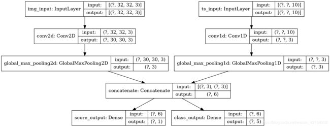
将数据传递到多输入、多输出模型

多输入、多输出模型示例：图像输入的shape（32，32，3）（即（height，width，channels））和时间序列输入的shape（None，10）（即（timesteps，features））。模型将从这两个输入组合计算出2个输出：“分数”（shape（1，））和五个类别（shape（5，））的概率分布。

from tensorflow import keras
from tensorflow.keras import layers

image_input = keras.Input(shape=(32, 32, 3), name='img_input')
timeseries_input = keras.Input(shape=(None, 10), name='ts_input')

x1 = layers.Conv2D(3, 3)(image_input)
x1 = layers.GlobalMaxPooling2D()(x1)

x2 = layers.Conv1D(3, 3)(timeseries_input)
x2 = layers.GlobalMaxPooling1D()(x2)

x = layers.concatenate([x1, x2])

score_output = layers.Dense(1, name='score_output')(x)
class_output = layers.Dense(5, name='class_output')(x)

model = keras.Model(inputs=[image_input, timeseries_input],
                    outputs=[score_output, class_output])
                    
keras.utils.plot_model(model, 'multi_input_and_output_model.png', show_shapes=True)

model.compile(
    optimizer=keras.optimizers.RMSprop(1e-3),
    loss=[keras.losses.MeanSquaredError(),
          keras.losses.CategoricalCrossentropy(from_logits=True)],
    metrics=[[keras.metrics.MeanAbsolutePercentageError(),
              keras.metrics.MeanAbsoluteError()],
             [keras.metrics.CategoricalAccuracy()]])

由于已经给输出层命名，可以通过dict指定每个输出损失和度量：

model.compile(
    optimizer=keras.optimizers.RMSprop(1e-3),
    loss={'score_output': keras.losses.MeanSquaredError(),
          'class_output': keras.losses.CategoricalCrossentropy(from_logits=True)},
    metrics={'score_output': [keras.metrics.MeanAbsolutePercentageError(),
                              keras.metrics.MeanAbsoluteError()],
             'class_output': [keras.metrics.CategoricalAccuracy()]})

使用loss-weights参数，可以为不同的output-specific losses赋予不同的权重，如下所示：

model.compile(
    optimizer=keras.optimizers.RMSprop(1e-3),
    loss={'score_output': keras.losses.MeanSquaredError(),
          'class_output': keras.losses.CategoricalCrossentropy(from_logits=True)},
    metrics={'score_output': [keras.metrics.MeanAbsolutePercentageError(),
                              keras.metrics.MeanAbsoluteError()],
             'class_output': [keras.metrics.CategoricalAccuracy()]},
    loss_weights={'score_output': 2., 'class_output': 1.})

如果这些输出用于预测，不用于训练，也可以选择不计算某些输出的损失：

# List loss version
model.compile(
    optimizer=keras.optimizers.RMSprop(1e-3),
    loss=[None, keras.losses.CategoricalCrossentropy(from_logits=True)])

# Or dict loss version
model.compile(
    optimizer=keras.optimizers.RMSprop(1e-3),
    loss={'class_output':keras.losses.CategoricalCrossentropy(from_logits=True)})

在fit中将数据传递给多输入多输出模型的方式与在compile中指定loss函数的方式类似：可以传递Numpy数组的列表（1:1映射到接收loss函数的输出）或dict将输出名称映射到Numpy训练数据数组。

model.compile(
    optimizer=keras.optimizers.RMSprop(1e-3),
    loss=[keras.losses.MeanSquaredError(),
          keras.losses.CategoricalCrossentropy(from_logits=True)])

# Generate dummy Numpy data
img_data = np.random.random_sample(size=(100, 32, 32, 3))
ts_data = np.random.random_sample(size=(100, 20, 10))
score_targets = np.random.random_sample(size=(100, 1))
class_targets = np.random.random_sample(size=(100, 5))

# Fit on lists
model.fit([img_data, ts_data], [score_targets, class_targets],
          batch_size=32,
          epochs=3)

# Alternatively, fit on dicts
model.fit({'img_input': img_data, 'ts_input': ts_data},
          {'score_output': score_targets, 'class_output': class_targets},
          batch_size=32,
          epochs=3)

Dataset的情况：

train_dataset = tf.data.Dataset.from_tensor_slices(
    ({'img_input': img_data, 'ts_input': ts_data},
     {'score_output': score_targets, 'class_output': class_targets}))
train_dataset = train_dataset.shuffle(buffer_size=1024).batch(64)

model.fit(train_dataset, epochs=3)

 

使用callbacks

Keras 中的 Callbacks 是在训练过程中的不同点调用的对象（在epoch开始时、批处理结束时、epoch结束时等），可用于实现以下行为：

	在训练期间的不同点进行验证
	定期检查模型或当模型超过某个精度阈值时
	训练趋于平稳时改变模型的学习率
	当训练似乎趋于平稳时，对顶层进行微调
	在训练结束或超过某个性能阈值时发送电子邮件或即时消息通知

回调可以作为列表在fit中调用：

callbacks = [
    keras.callbacks.EarlyStopping(
        # Stop training when `val_loss` is no longer improving
        monitor='val_loss',
        # "no longer improving" being defined as "no better than 1e-2 less"
        min_delta=1e-2,
        # "no longer improving" being further defined as "for at least 2 epochs"
        patience=2,
        verbose=1)
]
model.fit(x_train, y_train,
          epochs=20,
          batch_size=64,
          callbacks=callbacks,
          validation_split=0.2)

一些内置的callbacks：

1. ModelCheckpoint：定期保存模型。
2. EarlyStopping：当训练不再改进验证指标时，停止训练。
3. TensorBoard：定期编写可以在TensorBoard中可视化的模型日志。
4. CSVLogger：将损失和度量数据流到CSV文件。

自定义callback：

可以通过扩展基类keras.callbacks.Callback创建自定义callback。callback可以通过类属性self.model访问其关联的模型。

下面是一个简单的示例，保存了训练期间每批损失值的列表：

class LossHistory(keras.callbacks.Callback):

    def on_train_begin(self, logs):
        self.losses = []

    def on_batch_end(self, batch, logs):
        self.losses.append(logs.get('loss'))

 

Checkpointing 模型

在相对较大的数据集上训练模型时，必须经常保存模型的检查点。

实现这一点的最简单方法是使用ModelCheckpoint callback：

callbacks = [
    keras.callbacks.ModelCheckpoint(
        filepath='mymodel_{epoch}',
        # Path where to save the model
        # The two parameters below mean that we will overwrite
        # the current checkpoint if and only if
        # the `val_loss` score has improved.
        save_best_only=True,
        monitor='val_loss',
        verbose=1)
]
model.fit(x_train, y_train,
          epochs=3,
          batch_size=64,
          callbacks=callbacks,
          validation_split=0.2)

 

使用学习率表

在训练深度学习模型时，一个常见的模式是随着训练的进行逐渐减少学习。这通常被称为“学习率衰减”。

学习衰退时间表可以是静态的（预先固定的，作为当前epoch或当前批处理索引的函数），也可以是动态的（响应模型的当前行为，特别是验证损失）。

方法一：通过在优化器中将schedule对象作为learning_rate参数传递，可以轻松使用静态学习速率衰减表：

initial_learning_rate = 0.1
lr_schedule = keras.optimizers.schedules.ExponentialDecay(
    initial_learning_rate,
    decay_steps=100000,
    decay_rate=0.96,
    staircase=True)

optimizer = keras.optimizers.RMSprop(learning_rate=lr_schedule)

有几种内置的表可用：ExponentialDecay, PiecewiseConstantDecay, PolynomialDecay, 和InverseTimeDecay。

方法二：利用callbacks实现动态学习率表

 

训练期间loss和metrics的可视化

在训练期间，监视模型的最佳方法是使用TensorBoard，这是一个基于浏览器的应用程序，可以在本地运行：

1. 训练和评估时实时绘制loss和metrics
2. （可选）层激活直方图的可视化
3. （可选）Embedding层学习的嵌入空间的三维可视化

如果使用pip安装了TensorFlow，则应该能够从命令行启动TensorBoard：

tensorboard --logdir=/full_path_to_your_logs

使用TensorBoard callback：
在Keras模型和fit方法中使用TensorBoard的最简单方法是TensorBoard callback。

在最简单的情况下，只要指定callback要写入日志的位置，就可以：

tensorboard_cbk = keras.callbacks.TensorBoard(log_dir='/full_path_to_your_logs')
model.fit(dataset, epochs=10, callbacks=[tensorboard_cbk])

TensorBoard callback有许多有用的选项：

keras.callbacks.TensorBoard(
  log_dir='/full_path_to_your_logs',
  histogram_freq=0,  # How often to log histogram visualizations
  embeddings_freq=0,  # How often to log embedding visualizations
  update_freq='epoch')  # How often to write logs (default: once per epoch)

 

2：从头开始编写自己的训练和评估循环

使用GradientTape：端到端的示例

在GradientTape作用域内调用模型可以检索层的可训练权重相对于损失值的梯度。使用优化器实例，可以使用这些渐变来更新这些变量（可以使用model.trainable_weights检索).

# Get the model.
inputs = keras.Input(shape=(784,), name='digits')
x = layers.Dense(64, activation='relu', name='dense_1')(inputs)
x = layers.Dense(64, activation='relu', name='dense_2')(x)
outputs = layers.Dense(10, name='predictions')(x)
model = keras.Model(inputs=inputs, outputs=outputs)

# Instantiate an optimizer.
optimizer = keras.optimizers.SGD(learning_rate=1e-3)
# Instantiate a loss function.
loss_fn = keras.losses.SparseCategoricalCrossentropy(from_logits=True)

# Prepare the training dataset.
batch_size = 64
train_dataset = tf.data.Dataset.from_tensor_slices((x_train, y_train))
train_dataset = train_dataset.shuffle(buffer_size=1024).batch(batch_size)

epochs = 3
for epoch in range(epochs):
  print('Start of epoch %d' % (epoch,))

  # Iterate over the batches of the dataset.
  for step, (x_batch_train, y_batch_train) in enumerate(train_dataset):

    # Open a GradientTape to record the operations run
    # during the forward pass, which enables autodifferentiation.
    with tf.GradientTape() as tape:

      # Run the forward pass of the layer.
      # The operations that the layer applies
      # to its inputs are going to be recorded
      # on the GradientTape.
      logits = model(x_batch_train, training=True)  # Logits for this minibatch

      # Compute the loss value for this minibatch.
      loss_value = loss_fn(y_batch_train, logits)

    # Use the gradient tape to automatically retrieve
    # the gradients of the trainable variables with respect to the loss.
    grads = tape.gradient(loss_value, model.trainable_weights)

    # Run one step of gradient descent by updating
    # the value of the variables to minimize the loss.
    optimizer.apply_gradients(zip(grads, model.trainable_weights))

    # Log every 200 batches.
    if step % 200 == 0:
        print('Training loss (for one batch) at step %s: %s' % (step, float(loss_value)))
        print('Seen so far: %s samples' % ((step + 1) * 64))

 

参考资料

https://tensorflow.google.cn/guide/keras/custom_layers_and_models?hl=zh_cn