算法导论学习笔记15_最短路径

最短路径

  • 1. 单源最短路径
    • 1.1 Bellman-Ford算法
    • 1.2 有向无环图的单源最短路径
    • 1.3 Dijkstra算法
  • 2. 所有结点对的最短路径问题
    • 2.1 Floyd-Warshall算法
  • 3. 算法实现(C++)
    • 3.1 Bellman-Ford算法
    • 3.2 有向无环图的单源最短路径
    • 3.3 Dijkstra算法
    • 3.4 Floyd算法

1. 单源最短路径

1.1 Bellman-Ford算法

Bellman-Ford算法解决一般情况下的单源最短路径问题,这里边的权重可以是负值。当最短路径不存在是,Ford算法可以识别出来。

Bellman-Ford算法通过对边进行松弛操作来渐近地从源结点s到每个结点v的最短路径的估计值,直到该估计值与实际的最短路径权重相同时为止。

Bellman-Ford算法的伪代码如下:

BELLMAN-FORD(G, w, s)
	INITIALIZE-SINGLE-SOURCE(G.s)
	for i  = 1 to | G.V | - 1
		for each edge(u, v)∈G.E
			RELAX(u, v, w)
	for each edge(u, v) ∈ G.E
		if v.d > u.d + w(u, v)
			return FALSE;
	return TRUE;

其中,结点u包含两个额外属性:dp,分别表示该结点到源结点s的距离的估计和该结点在最短路径上的父结点的估计。

因此,INITIALIZE-SINGLE-SOURCE的操作是对这两个属性进行初始化:

INITIALIZE-SINGLE-SOURCE(G.s)
	for each vertex v ∈ G.V
		v.d = ∞
		v.p = NIL
	s.d = 0

此外,上述RELAX就是求最短路径中最常用的松弛操作:

RELAX(u, v, w)
	if v.d > u.d + w
		v.d = u.d + w
		v.p = u

因此,Bellman-Ford算法实际上就是对所有的边进行了N-1边松弛操作,最后求得源结点s到任意结点u的最短距离u.d

Bellman-Ford算法的总运行时间为O(VE)

1.2 有向无环图的单源最短路径

Bellman-Ford解决的是一般情况下的单源最短路径,然而很多时候图满足一些条件,例如不包含环,不包含负值等。这个时候可对算法效率进行提升。

根据结点的拓扑排序来对带权重的有向无环图进行边的松弛操作,可以在θ(V + E)时间内计算出从单个源结点到所有结点之间的最短路径。

算法的伪代码如下:

DAG-SHORTEST-PATHS(G, w, s)
	topologically sort the vertices of G
	INITALIZE-SINGLE-SOURCE(G, s)
	for each vertex u, taken in topoigitcally soted order
		for each vertex v ∈ G.Adj[u]
			RELAX(u, v, w)

可以看出,上述代码中松弛的次数从Bellman-Ford算法的|G.V - 1| * |G.E|次减少到了|G.E|次。而增加的拓扑排序操作的时间复杂度为θ(V + E)。因此,该算法的总运行时间为θ(V + E)

1.3 Dijkstra算法

当图满足所有的边的权重不为负值时(实际上很多情况下都满足这个性质),Dijkstra算法往往性能比Bellman-Ford的性能好。

Dijkstra算法在运行过程中维护的关键信息是一组结点集合S。从源结点s到该集合中每个结点之间的最短路径已经找到。算法重复从结点集V-S中选择最短路径估计最小的结点u,将u加入到集合S,然后对所有从u发出的边进行松弛。

Dijkstra算法的伪代码如下:

DIJKSTRA(G, w, s)
	INITIALIZE-SINGLE-SOURCE(G, s)
	S = φ
	Q = G.V
	while Q ≠ φ
		u = EXTRACT-MIN(Q)
		S = S ∪ {u}
		for each vertex in G.Adj[u]
			RELAX(u, v, w)

因为Dijkstra算法总是选择集合V-S中最近的结点来加入到集合S中,该算法使用的是贪心策略。

值得注意的是,为了提升算法的性能,上述代码中的Q往往用优先队列实现,队列的头部保留着集合V-S中路径估计最小的结点。

此外,由于松弛操作会改变集合V-S中的结点的dp属性,此时应该更新优先队列Q,因此这里的松弛操作与Bellman-Ford算法中的松弛操作会略有不同,具体可见附录代码。

2. 所有结点对的最短路径问题

2.1 Floyd-Warshall算法

Floyd-Warshall算法是一种动态规划算法,它可以计算所有结点之间的最短路径。

伪代码如下:

FLOYD-WARSAHLL(w)
	n = W.rows
	Initialize distance matrix D
	for k = 1 to n
		for i = 1 to n
			for j = 1 to n
				Dij = min(Dij, Dik + Dkj)
	return D

可以看到,Floyd算法非常的简洁,主程序只有三层的for循环,通过自底向上计算最短路径,最后得到所以结点之间的最短路径。

3. 算法实现(C++)

3.1 Bellman-Ford算法

对于如下带环和负值的有向图:

算法导论学习笔记15_最短路径_第1张图片

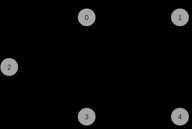
利用Bellman-Ford算法求解从以结点2为源的的最短路径代码如下:

#include 
#include 
#include 
#include 

using namespace std;

struct Vertex {
	Vertex(int distance, int vid, shared_ptr<Vertex> parent) :
		d(distance), id(vid), p(parent) {}
	int d;
	int id;
	shared_ptr<Vertex> p = nullptr;
};
struct Edge {
	shared_ptr<Vertex> u = nullptr;
	shared_ptr<Vertex> v = nullptr;
	int w;
};
struct Graph {
	vector<shared_ptr<Vertex>> V;
	vector<Edge> E;
};
class Ford {
public:
	explicit Ford(Graph& graph) : G(graph) {};
	bool bellman_ford(unsigned s) {
		init_single_source(s);
		for (int i = 0; i < G.V.size() - 1; ++i) {
			for (Edge& e : G.E) {
				relax(e.u, e.v, e.w);
			}
		}
		for (const Edge& e : G.E) {
			if (e.v->d > e.u->d + e.w)
				return false;
		}
		return true;
	}
	void print_path(unsigned i) {
		shared_ptr<Vertex> v = G.V[i];
		cout << i;
		while (v->p) {
			cout << " <- " << v->p->id;
			v = v->p;
		}
		cout << endl;
	}
private:
	Graph& G;
	void init_single_source(unsigned s) {
		G.V[s]->d = 0;
	}
	void relax(shared_ptr<Vertex> u, shared_ptr<Vertex> v, int w) {
		if (v->d > u->d + w) {
			v->d = u->d + w;
			v->p = u;
		}
	}
};

Graph make_graph(vector<vector<pair<int, int>>> vec) {
	Graph G;
	// Load Verticies
	for (int i = 0; i < vec.size(); ++i) {
		G.V.push_back(make_shared<Vertex>( 99999, i, nullptr));
	}
	// Load Edges
	for (int i = 0; i < vec.size(); ++i) {
		shared_ptr<Vertex> u = G.V[i];
		for (int j = 0; j < vec[i].size(); ++j) {
			shared_ptr<Vertex> v = G.V[vec[i][j].first];
			int w = vec[i][j].second;
			G.E.push_back({ u, v, w });
		}
	}
	return G;
}
int main(void) {
	vector<vector<pair<int, int>>> vec = {
		{{1, 5}, {3, 8}, {4, -4}},
		{{0, -2}},
		{{0, 6}, {3, 7}},
		{{1, -3}, {4, 9}},
		{{2, 2}, {1, 7}}
	};
	Graph G = make_graph(vec);
	Ford F(G);
	F.bellman_ford(2);
	for (int i = 0; i < vec.size(); ++i)
		F.print_path(i);
	return 0;
}

输出为:

0 <- 1 <- 3 <- 2
1 <- 3 <- 2
2
3 <- 2
4 <- 0 <- 1 <- 3 <- 2

3.2 有向无环图的单源最短路径

对于下面带负值的有向无环图:

算法导论学习笔记15_最短路径_第2张图片

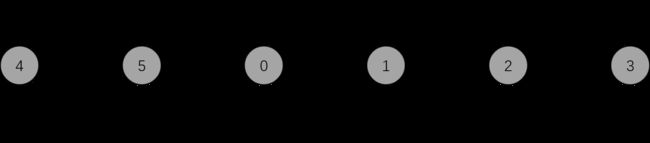
可以首先对图中的所有结点进行拓扑排序,然后对于所有的结点,按照拓扑的顺序对其之后的所有边进行松弛操作。

代码如下:

#include 
#include 
#include 
#include 
#include 
using namespace std;
struct Vertex {
	Vertex(int vd, int vid, int vdepth, shared_ptr<Vertex> vp):
		d(vd), id(vid), depth(vdepth), p(vp){}
	int d;	
	int id;
	int depth;
	shared_ptr<Vertex> p = nullptr;
};
struct Edge {
	shared_ptr<Vertex> u;
	shared_ptr<Vertex> v;
	int w;
};
using ADJ = vector<Edge>;
struct Graph {
	vector<shared_ptr<Vertex>> V;
	vector<ADJ> Adj;
};
class DAG {
public:
	explicit DAG(Graph& graph) : G(graph) {};
	void init_single_source(unsigned id) {
		for (int i = 0; i < G.Adj.size(); ++i)
			if (G.V[i]->id == id)
				G.V[i]->d = 0;
	}
	void relax(shared_ptr<Vertex> u, shared_ptr<Vertex> v, int w) {
		if (v->d > u->d + w) {
			v->d = u->d + w;
			v->p = u;
		}
	}
	bool shortest_paths(unsigned s) {
		top_sort();
		init_single_source(s);
		for (int i = 0; i < G.V.size() - 1; ++i) {
			for (int j = 0; j < G.Adj[G.V[i]->id].size(); ++j) {
				shared_ptr<Vertex> u = G.Adj[G.V[i]->id][j].u;
				shared_ptr<Vertex> v = G.Adj[G.V[i]->id][j].v;
				int w = G.Adj[G.V[i]->id][j].w;
				relax(u, v, w);
			}
		}
		return true;
	}
	void top_sort() {
		for (shared_ptr<Vertex> vp : G.V) {
			vp->depth = dfs(vp->id);
		}
		sort(G.V.begin(), G.V.end(), 
			[](const auto& a, const auto& b) { return a->depth > b->depth; });
	}
	int dfs(unsigned id) {
		if (G.V[id]->depth != 0) return G.V[id]->depth;
		int max_len = 1;
		for (int j = 0; j < G.Adj[id].size(); ++j)
			max_len = max(max_len, 1 + dfs(G.Adj[id][j].v->id));
		return max_len;
	}
	void print_path(unsigned id) {
		shared_ptr<Vertex> v = G.V[id];
		cout << v->id;
		while (v->p) {
			cout << " <- " << v->p->id;
			v = v->p;
		}
		cout << endl;
	}
private:
	Graph& G;
};

Graph make_graph(vector<vector<pair<int, int>>> vec) {
	Graph G;
	// Load Verticies
	for (int i = 0; i < vec.size(); ++i) {
		shared_ptr<Vertex> u = make_shared<Vertex>(99999, i, 0, nullptr);
		G.V.push_back(u);
	}
	// Load Edges
	for (int i = 0; i < vec.size(); ++i) {
		shared_ptr<Vertex> u = G.V[i];
		G.Adj.push_back({});
		for (int j = 0; j < vec[i].size(); ++j) {
			shared_ptr<Vertex> v = G.V[vec[i][j].first];
			int w = vec[i][j].second;
			G.Adj[i].push_back({u, v, w});
		}
	}
	return G;
}
int main(void) {
	vector<vector<pair<int, int>>> vec = {
		{{1, 7}, {2, 4}, {3, 2}},
		{{2, -1}, {3, 1}},
		{{3, -2}},
		{},
		{{5, 5}, {0, 3}},
		{{0, 2}, {1, 6}}
	};
	Graph G = make_graph(vec);
	DAG D(G);
	D.shortest_paths(4);
	for (int i = 0; i < vec.size(); ++i)
		D.print_path(i);
	return 0;
}

输出为:

4
5 <- 4
0 <- 4
1 <- 0 <- 4
2 <- 0 <- 4
3 <- 0 <- 4

3.3 Dijkstra算法

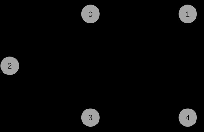
Dijkstra可用于不带负权值的图,例如下图:

算法导论学习笔记15_最短路径_第3张图片

代码:

#include 
#include 
#include 
#include 
#include 
#include 

using namespace std;

struct Vertex {
	// Vertex datastruct
	Vertex(int vid, int vd, shared_ptr<Vertex> vp) :
		id(vid), d(vd), p(vp){}
	int id;
	int d;
	shared_ptr<Vertex> p;
};
struct Edge {
	// Edge datastruct
	shared_ptr<Vertex> u;
	shared_ptr<Vertex> v;
	int w;
};
using ADJ = unordered_map<int, vector<Edge>>;
struct Graph {
	// Graph datastruct
	vector<shared_ptr<Vertex>> V;
	ADJ Adj;
};
bool operator<(const shared_ptr<Vertex> a, const shared_ptr<Vertex> b) {
	// Overload the "<" operator for priority_queue
	// To implement the "big-endian" priority_queue, return ">" rather than "<"
	return a->d > b->d;
}
class Dijkstra {
public:
	Dijkstra(Graph& Graph) : G(Graph) {}
	void initialize_single_source(int id) {
		// Initialize single source
		for (int i = 0; i < G.V.size(); ++i)
			if (G.V[i]->id == id)
				G.V[i]->d = 0;
	}
	void relax(priority_queue<shared_ptr<Vertex>>& Q, Edge& edge) {
		// Relaxation operation
		if (edge.v->d > edge.u->d + edge.w) {
			edge.v->d = edge.u->d + edge.w;
			edge.v->p = edge.u;
			Q.push(edge.v);
		}
	}
	void shortest_paths(int id) {
		// Dijkstra algorithm main process
		initialize_single_source(id);
		vector<int> S(G.V.size(), 0);
		priority_queue<shared_ptr<Vertex>> Q;
		Q.push(G.V[id]);
		while (!Q.empty()) {
			shared_ptr<Vertex> u = Q.top(); Q.pop();
			if (S[u->id]) continue;
			S[u->id] = 1;
			for (int i = 0; i < G.Adj[u->id].size(); ++i)
				relax(Q, G.Adj[u->id][i]);
		}
	}
	void print_path(unsigned i) {
		// Print the path backwards
		shared_ptr<Vertex> v = G.V[i];
		cout << v->id;
		while (v->p) {
			cout << " <- ";
			cout << v->p->id;
			v = v->p;
		}
		cout << endl;
	}
private:
	Graph& G;
};
Graph make_graph(const vector<vector<pair<int, int>>>& vec) {
	Graph G;
	// Load vertexes
	for (int i = 0; i < vec.size(); ++i) {
		shared_ptr<Vertex> u = make_shared<Vertex>(i, 99999, nullptr);
		G.V.push_back(u);
		G.Adj[u->id] = {};
	}
	// Load edges
	for (int i = 0; i < vec.size(); ++i) {
		shared_ptr<Vertex> u = G.V[i];
		for (int j = 0; j < vec[i].size(); ++j) {
			shared_ptr<Vertex> v = G.V[vec[i][j].first];
			int w = vec[i][j].second;
			G.Adj[u->id].push_back({ u, v, w });
		}
	}
	return G;
}
int main(void) {
	vector<vector<pair<int, int>>> vec = {
		{{1, 1}, {3, 2}},
		{{4, 4}},
		{{0, 10}, {3, 5}},
		{{0, 2}, {1, 9}, {4, 2}},
		{{1, 6}, {2, 7}} };
	Graph G = make_graph(vec);
	Dijkstra D(G);
	D.shortest_paths(2);
	for (int i = 0; i < G.V.size(); ++i)
		D.print_path(i);
	return 0;
}

输出为:

0 <- 3 <- 2
1 <- 0 <- 3 <- 2
2
3 <- 2
4 <- 3 <- 2

3.4 Floyd算法

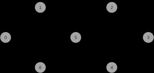
Floyd算法可用于计算图中所有结点之间的距离, 如下图:

算法导论学习笔记15_最短路径_第4张图片

代码:

#include 
#include 
#include 

using namespace std;

class Floyd {
public:
	explicit Floyd(vector<vector<int>> map, int n) {
		// Initialize matrix d and matrix p with value that is large enough
		d = vector<vector<int>>(n, vector<int>(n, 99999));
		p = d;
		for (int i = 0; i < n; ++i) d[i][i] = 0;
		for (const auto& path : map) {
			d[path[0]][path[1]] = d[path[1]][path[0]] = path[2];
		}
	}
	void shortest_paths() {
		// Floyd algorithm main process
		int n = d.size();
		for (int k = 0; k < n; ++k)
			for (int i = 0; i < n; ++i)
				for (int j = 0; j < n; ++j)
					if (d[i][k] + d[k][j] < d[i][j]) {
						d[i][j] = d[i][k] + d[k][j];
						p[i][j] = p[j][i] = k;
					}
	}
	void dfs(int start, int end, vector<int>& path) {
		// In order traverse
		if (p[start][end] == 99999) return;
		dfs(start, p[start][end], path);
		path.push_back(p[start][end]);
		dfs(p[start][end], end, path);
	}
	void print_path(int start, int end){
		// print shortest path for giving start and end
		vector<int> path;
		dfs(start, end, path);
		cout << start << " ";
		for (const auto& p : path)
			cout << p << " ";
		cout << end << endl;
	}
	void print_pd() {
		// print matrix p and matrix d
		for (int i = 0; i < p.size(); ++i) {
			for (int j = 0; j < p.size(); ++j)
				cout << p[i][j] << "\t";
			cout << endl;
		}
		cout << endl;
		for (int i = 0; i < d.size(); ++i) {
			for (int j = 0; j < d.size(); ++j)
				cout << d[i][j] << "\t";
			cout << endl;
		}
	}
private:
	vector<vector<int>> d, p;
};


int main(void) {
	vector<vector<int>> map = {
		{0, 1, 12}, {0, 5, 16}, {0, 6, 14}, {1, 2, 10}, {1, 5, 7}, 
		{6, 4, 8},  {6, 5, 9},  {5, 2, 6},  {5, 4, 2},  {2, 4, 5}, 
	    {2, 3, 3},  {3, 4, 4}
	};
	Floyd F(map, 7);
	F.shortest_paths();
	//F.print_pd();
	F.print_path(0, 3);
	return 0;
}

输出为:

0 -> 5 -> 4 -> 3

你可能感兴趣的:(算法)