探索seurat包

一、了解包的基本内容

1. 加载

if(!require(Seurat))
  BiocManager::install('Seurat')
if(!require(scRNAseq))
  BiocManager::install('scRNAseq')

2. 基本信息

• 参考
  https://satijalab.org/seurat/v3.1/pbmc3k_tutorial.html

• 输入数据
  a. cellranger 输出的10X数据
  b. 未经过标准化的数据：raw counts /TPMs

二、使用

1. 导入数据

data(fluidigm)
assay(fluidigm) <- assays(fluidigm)$rsem_counts
ct <- floor(assays(fluidigm)$rsem_counts)

2. 创建对象和基本操作

1）检查数据

meta <- as.data.frame(colData(fluidigm))  #细胞相关信息
counts <- ct #表达矩阵
identical(rownames(meta),colnames(counts))#检查counts的列名和meta的行名是否保持一致
fivenum(apply(ct,1,function(x) sum(x>0))) #基因表达的细胞数目
fivenum(apply(ct,2,function(x) sum(x>0) ))#细胞表达的基因数目

由上图可见有至少25%的基因不表达，至少50%的基因表达的细胞数目不超过5个；细胞表达的基因数目多于1418个

2）创建对象

sce <- CreateSeuratObject(counts  = counts, #表达矩阵
                           meta.data =meta,  #细胞信息
                           min.cells = 3,    #基因表达的最少细胞数目
                           min.features  = 200,#细胞表达的最少基因数目
                           project = "sce") #项目名称

过滤了11599个基因和0个细胞

3）查看对象内容

str(sce)

在后续操作时默认使用active.assay，也可以使用assay参数指定使用的表达矩阵

4）调用对象内容

head(sce@assays$RNA@counts[,1:4])

sce存储的表达矩阵是类矩阵，只能使用Matrix包的函数进行操作

5）向对象插入内容

为元信息增加线粒体基因的比例，如果线粒体基因所占比例过高，意味着这可能是死细胞

mito.genes <- grep(pattern = "^MT-", x = rownames(x = sce@assays$RNA@data), value = TRUE) #这个例子的表达矩阵里面没有线粒体基因
percent.mito <- Matrix::colSums(sce@assays$RNA@counts[mito.genes, ]) / Matrix::colSums(sce@assays$RNA@counts) 
sce <- AddMetaData(object = sce, metadata = percent.mito,col.name = "percent.mito")

在 meta.data元素里新增了一列

6）可视化对象内容

a. 小提琴图

VlnPlot(object = sce, features = c("nCount_RNA", "nFeature_RNA", "percent.mito"), group.by = 'Biological_Condition')

不同类型的细胞测序深度和表达的基因数目均有差异

b. 散点图

tail(sort(Matrix::rowSums(sce@assays$RNA)))#高表达基因

plot1 <- FeatureScatter(sce, feature1 = "SOX11", feature2 = "EEF1A1",group.by = "Biological_Condition") #基因间关系
plot2 <- FeatureScatter(sce, feature1 = "nCount_RNA", feature2 = "nFeature_RNA",group.by = "Biological_Condition") #细胞信息间关系
CombinePlots(plots = list(plot1, plot2)) #展示在同一页面

3. 归一化

sce1<-sce #备份
sce <- NormalizeData(object = sce, 
                     normalization.method = "LogNormalize",  #文库大小归一化及log
                     scale.factor = 10000 #文库大小
                     )

归一化后的表达矩阵存储在data元素里

4. 挑选高变异基因

使用数据：counts，而不是data

sce <- FindVariableFeatures(sce, selection.method = "vst", nfeatures = 2000)

2000个高变异基因存储在var.features元素里
优化函数：sctransform

• 可视化

plot1 <- VariableFeaturePlot(sce)
top10 <- head(VariableFeatures(sce), 10) #挑选变化最大的10个基因
plot2 <- LabelPoints(plot = plot1, points = top10, repel = TRUE,xnudge=0,ynudge=0) #标注基因名
CombinePlots(plots = list(plot1, plot2),legend = "bottom")

5. 标准化及去除混杂因素影响

a. seurat包要求PCA之前必须标准化
b. 使用数据：data

sce <- ScaleData(sce,
				features = NULL,#默认使用高变异基因进行标准化
				#vars.to.regress="nUMI"#去除文库大小的影响
				)
sce[["RNA"]]@scale.data[1:4,1:4]

标准化后的矩阵存储在scale.data元素里

6. 降维

a. 使用高变异基因进行降维，从而可以加快计算速度
b. 降维结果存储在reductions元素里
c. 使用少量的PC既能关注到关键的生物学差异，又能够不引入更多的技术差异，相当于一种保守性的做法
d. 使用scale.data元素

1）PCA

sce <- RunPCA(sce, 
			  features = VariableFeatures(object = sce),#使用高变异基因降维
              ndims.print=1:2,nfeatures.print=5 #打印出来的维度和基因数目
              )

• 可视化
  a. 基因对每个主成分的重要性占比情况

VizDimLoadings(sce, dims = 1:2, reduction = "pca")

b. 主成分图

DimPlot(sce, reduction = "pca",group.by = "Biological_Condition")

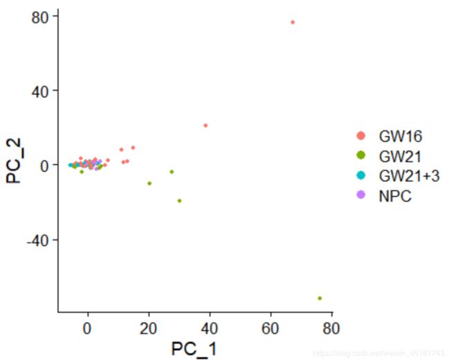
NPC和GW细胞完全混合在一起，说明挑选高变异基因的方法不对，导致数据分布与生物学认知不同，按道理来说应该要更换方法重新挑选高变异基因，但因为只是探索所以用该套数据继续往下做

c. 热图

DimHeatmap(sce, dims = 1, balanced = TRUE)

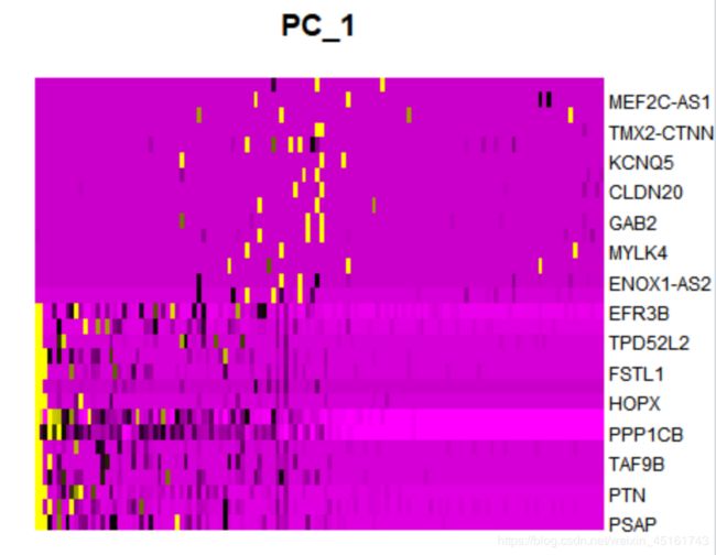
主成分越前的贡献基因按道理来说在样本里的差异性越大，但是因为挑选的高变异基因不太对，所以体现不出这种差异
正确图：

d. 挑选主成分

ElbowPlot(sce)

一般取点保持平衡趋势的前几个主成分，在上图应取前20个主成分

2）UMAP

sce <- RunUMAP(sce, dims = 1:20) #取PCA前20个主成分进行计算，加快速度
DimPlot(sce, reduction = "umap",group.by = "Biological_Condition")

说明该套数据存在技术变异，影响了可视化结果。从文献中可知该套数据使用了两种测序深度，所以可以推测进行下游分析前需去除测序深度变异（目前没有找到一个细胞属性可以很好地进行批次处理）

3）tSNE

sce <- RunTSNE(object = sce, dims.use = 1:20)
DimPlot(sce, reduction = "tsne",group.by = "Biological_Condition")

效果没有umap好

7. 聚类

• 确定邻域

sce <- FindNeighbors(sce, dims = 1:20)

存储在graph元素里

• 分类

sce <- FindClusters(sce,resolution = 1.2) #resolution值越大分组越多
head(Idents(sce), 5)

存储在meta.data元素里

8. 确定差异表达基因

运行速度很慢

• 仅确定某类

marker1<-FindMarkers(sce, ident.1 = 1)
head(marker1)

• 确定所有类

marker<-FindAllMarkers(sce)

• 可视化

1. 在降维图上可视化基因表达

FeaturePlot(sce, features ="RPL18AP3" )

2. 热图

library(dplyr)
top10 <- marker %>% group_by(cluster) %>% top_n(n = 10, wt = avg_logFC)
DoHeatmap(sce, features = top10$gene) + NoLegend() #无图例

3. 在降维图上进行注释

new.cluster.ids <-top10$gene
names(new.cluster.ids)<-rep(0:3, each = 10)
sce <- RenameIdents(sce, new.cluster.ids)

只使用了new.cluster.ids中每一类的第一个基因修改ident

DimPlot(sce, reduction = "pca", label = TRUE, pt.size = 0.5) + NoLegend()

9. 总结

a. 创建对象所需元素： counts矩阵

b. 归一化函数
NormalizeData ：文库大小归一化和log化
ScaleData ：标准化和技术差异校正

c. 挑选基因函数
FindVariableGenes ：挑选适合进行下游分析的基因集
FindAllMarkers：挑选各个亚群的标志基因

d. 降维函数： RunPCA，RunTSNE，RunUMAP

e. 可视化基因函数：
FeaturePlot：不同基因在所有细胞的表达量
VlnPlot：不同基因在不同分群的表达量
DoHeatmap：选定基因集绘制热图