机器学习之算法-梯度下降画图

梯度下降

损失函数公式:

转换为矩阵形式为:


用到的代码:

import numpy as np
import os
#画图
%matplotlib inline
import matplotlib.pyplot as plt

#随机种子
np.random.seed(42)  #西瓜,绿豆 无所谓多少

#保存图像
PROJECT_ROOT_DIT = "."
MODEL_ID = "linear_models"  #线性模型


def save_fig(fig_id,tight_layout = True):  #定义一个保存图像的函数  自动填充画布tight_layout
    path = os.path.join(PROJECT_ROOT_DIT,'images',MODEL_ID,fig_id + ".png") #指定保存图像的路劲 手动创建 当前目录下的images文件夹下的model_id文件夹
    print("Saving figure",fig_id)  #提示函数,正在保存图片
    plt.savefig(path,format = 'png',dpi = 300) #保存图片 (需要指定保存路径,保存格式,清晰度)
    
# "./images/linear_models/xx.png"
#把讨厌的警告信息过滤掉
import warnings
warnings.filterwarnings(action = 'ignore',message = "^internal gelsd")

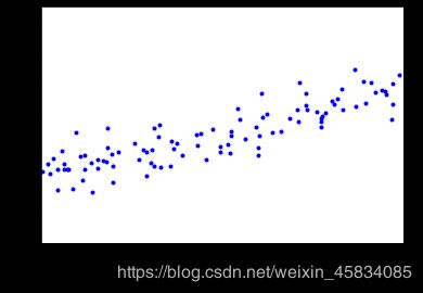
X = 2 * np.random.rand(100,1)  #生成训练数据(特征部分)
y = 4 + 3 * X + np.random.randn(100,1)#生成训练数据(标签部分)

plt.plot(X,y,'b.') #画图
plt.xlabel("$x_1$",fontsize = 18)
plt.ylabel("$y$",rotation = 0,fontsize = 18) # rotation 旋转角度
plt.axis([0,2,0,15]) #x 轴的范围是0-2 y轴的范围是0-15
save_fig("generated_data_plot") #调用保存图片函数save_fig
plt.show()

#添加新特征
X_b = np.c_[np.ones((100,1)),X]  # 添加一列
X_b

# 创建测试数据
X_new = np.array([[0],[2]])
X_new_b = np.c_[np.ones((2,1)),X_new]

from sklearn.linear_model import LinearRegression #从 sklearn包里导入线性回归模型
lin_reg = LinearRegression() #创建线性回归对象
lin_reg.fit(X,y) #拟合训练数据
lin_reg.intercept_,lin_reg.coef_ #输出截距,斜率

lin_reg.predict(X_new) #对测试集进行预测

批量梯度下降求解线性回归

eta = 0.1 #a法
n_iterations = 1000  #迭代次数固定
m = 100  
theta = np.random.randn(2,1)

for iterations in range(n_iterations):
    gradients = 1/m * X_b.T.dot(X_b.dot(theta)-y)  #dot 矩阵的乘积  梯度
    theta = theta - eta * gradients #更新theta值

theta_path_bgd = []

def plot_gradient_descent(theta,eta,theta_path = None):
    m = len(X_b)
    plt.plot(X,y,'b.')
    n_iterations = 1000
    for iterations in range(n_iterations):
        if iterations < 10:  #画蓝色线
            y_predict = X_new_b.dot(theta)
            style = "b-"
            plt.plot(X_new,y_predict,style)
        gradients = 2/m * X_b.T.dot(X_b.dot(theta)-y)  #dot 矩阵的乘积
        theta = theta - eta * gradients
        if theta_path is not None:  #保存更新的theta_path的值
            theta_path.append(theta)
    plt.xlabel("$x_1$",fontsize = 18)
    plt.axis([0,2,0,15]) #x 轴的范围是0-2 y轴的范围是0-15
    plt.title(r"$\eta = {}$".format(eta),fontsize = 16) #保存图片

#随机种子
np.random.seed(42)
theta = np.random.randn(2,1) # random initialization

plt.figure(figsize = (10,4))
plt.subplot(131);plot_gradient_descent(theta,eta=0.02)
plt.ylabel("$y$",rotation = 0,fontsize = 18)
plt.subplot(132);plot_gradient_descent(theta,eta=0.1,theta_path=theta_path_bgd)   #调用函数
plt.subplot(133);plot_gradient_descent(theta,eta=0.5)
# 第一个代表行数，第二个代表列数，第三个代表索引位置。
# 举个列子：plt.subplot(2, 3, 5) 和 plt.subplot(235) 是一样一样的。需要注意的是所有的数字不能超过10
save_fig("gradient_descent_plot")  #调用保存图片函数save_fig
plt.show()

随机梯度下降法

具体过程

theta_path_sgd = []
m = len(X_b)
np.random.seed(42)

n_epochs = 50

theta = np.random.randn(2,1)  #随机初始化

for epoch in range(n_epochs):
    for i in range(m):
        if epoch == 0 and i < 20:
            y_predict = X_new_b.dot(theta)
            style = "p-"
            plt.plot(X_new,y_predict,style)
        random_index = np.random.randint(m)
        xi = X_b[random_index:random_index + 1]
        yi = y[random_index:random_index + 1]
        gradients = 2 * xi.T.dot(xi.dot(theta)-yi)  #dot 矩阵的乘积
        eta = 0.1
        theta = theta - eta * gradients
        theta_path_sgd.append(theta)
plt.plot(X,y,'b.')
plt.xlabel("$x_1$",fontsize = 18)
plt.ylabel("$y$",rotation = 0,fontsize =18)
plt.axis([0,2,0,15]) #x 轴的范围是0-2 y轴的范围是0-15
save_fig("sgd_plot")  #调用保存图片函数save_fig
plt.show()

直接导包写代码

from sklearn.linear_model import SGDRegressor
sgd_reg = SGDRegressor(max_iter=50,tol=-np.infty,penalty=None,eta0=0.1,random_state=42)   #最大迭代次数  惩罚(结构风险)=None 不考虑l1 l2
sgd_reg.fit(X,y.ravel())

sgd_reg.intercept_,sgd_reg.coef_  #输出截距,斜率

小批量梯度下降Mini-batch gradient descent

theta_path_mgd = []
n_iterations = 50
minibatch_size = 20

np.random.seed(42)
theta = np.random.randn(2,1)


for epoch in range(n_iterations):
    shuffled_indices = np.random.permutation(m)  #洗牌
    X_b_shuffled = X_b[shuffled_indices]
    y_shuffled = y[shuffled_indices]
    for i in range(0,m,minibatch_size):
        xi = X_b_shuffled[i:i+minibatch_size]
        yi = y_shuffled[i:i+minibatch_size]
        gradients = 2/minibatch_size *  xi.T.dot(xi.dot(theta)-yi)  #dot 矩阵的乘积
        eta = 0.1
        theta = theta - eta * gradients
        theta_path_mgd.append(theta)

theta

theta_path_bgd = np.array(theta_path_bgd)
theta_path_sgd = np.array(theta_path_sgd)
theta_path_mgd = np.array(theta_path_mgd)

plt.figure(figsize=(7,4))
plt.plot(theta_path_sgd[:,0],theta_path_sgd[:,1],"r-s",linewidth=1,label="Stochastic")
plt.plot(theta_path_mgd[:,0],theta_path_mgd[:,1],"g-+",linewidth=2,label="Mini-batch")
plt.plot(theta_path_bgd[:,0],theta_path_bgd[:,1],"b-o",linewidth=3,label="Batch")
plt.legend(loc="upper left",fontsize=16)
plt.xlabel(r"$\theta_0$",fontsize = 20)
plt.ylabel(r"$\theta_1$",fontsize = 20,rotation = 0)
plt.axis([2.5,4.5,2.3,3.9])
save_fig("gradient_descent_paths_plot")
plt.show()