今天在看看 Kaggle 有沒有什麼新的玩意,看到一個德國的二手車的資料集,剛好前陣子有個車廠的業務說他在德國住10幾年,而且我問了他一些有關德國的車廠問題,他的言論我是保持懷疑態度,剛好也可以複習並綜合Kaggle專家們的統計手法,並使用 Tensorflow 的迴歸預測來塑模。
** 資料 **
- Kaggle - Used cars database
** 資訊技術 **
- R: ggplot2, data.table, dplyr, Hmisc
- Python: pandas, tensorflow, sklearn
** 資料探索 **
先看一些基本的資料屬性值,在 R 中可以直接用 summary 或是使用 其他 package 來觀察,個人偏好 Hmisc:
library('Hmisc')
describe(autos)
共有 20 個屬性,371,824筆資料,每個數值資料屬性值的描述會如下格式:
----------------------------------------------------------------------------------------------------------
price
       n  missing distinct     Info     Mean      Gmd      .05      .10      .25      .50      .75
  371824        0     5597        1    17286    29882      200      500     1150     2950     7200
     .90      .95
   14000    19788

lowest :          0          1          2          3          4
highest:   32545461   74185296   99000000   99999999 2147483647

0 (371783, 1), 2e+07 (22, 0), 4e+07 (1, 0), 8e+07 (1, 0), 1e+08 (16, 0), 2.14e+09 (1, 0)
----------------------------------------------------------------------------------------------------------
觀察到幾個比較是極端值的狀況:
- Price 的最低值與最高值過度極端,以歐元計價,則 2,147,483,647 及 99,999,999 這幾個數字過度極端,將其範圍限定在較為合理的區間
- Missing Values: vehicleType, gearbox, model, fuelType, notRepairedDamage, 這裡我採用直接 drop 方式
- yearOfRegistration的最小值有 1000 年?最高值有 9999 年?將其範圍限定在較為合理的範圍
- powerPS: 馬力值到一萬是比較誇張, 將其範圍限定在合理的均數以下
經過 dplyr 整理, 取得 192,039 筆有效資料:
autos <- data.table(autos %>%
                      filter(yearOfRegistration >= 2000 & yearOfRegistration < 2017) %>%
                      filter(price <= 100000 & price >= 100) %>%
                      filter(powerPS <= 1000) %>%
                      filter(!is.na(vehicleType)) %>%
                      filter(!is.na(gearbox)) %>%
                      filter(!is.na(model)) %>%
                      filter(!is.na(fuelType)) %>%
                      filter(!is.na(notRepairedDamage)) )
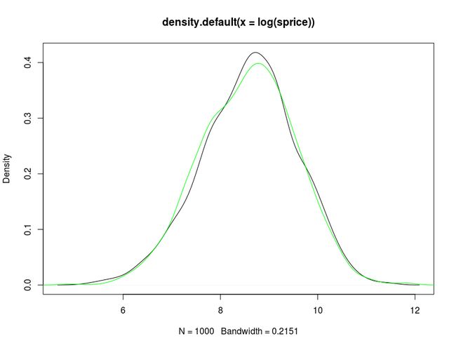
Orges Leka 提出價格分佈是一個對數常態分配,Price distribution is log-normal,我認同價格的特性應是如此,並檢測 192,125 筆資料是否也有此特性,在 ks 檢定中也符合顯著性(p-value = 0.828):
sprice <- sample(autos$price,1000); plot(density(log(sprice)))
rn <- rnorm(length(sprice),mean=mean(log(sprice)),sd=sd(log(sprice)))
lines(density( rn),col="green")
這裡我要驗證業務先生的說詞,故將不同車廠的數量排序,再弄張圖來視覺化:
brands <- autos[, .N, by=list(brand)]
setorderv(brands, c('N'), c(-1))

ggplot(brands[0:10, ,], aes(x=brand, y=N, colour=brand, fill=brand))  +
  geom_bar(stat="identity")
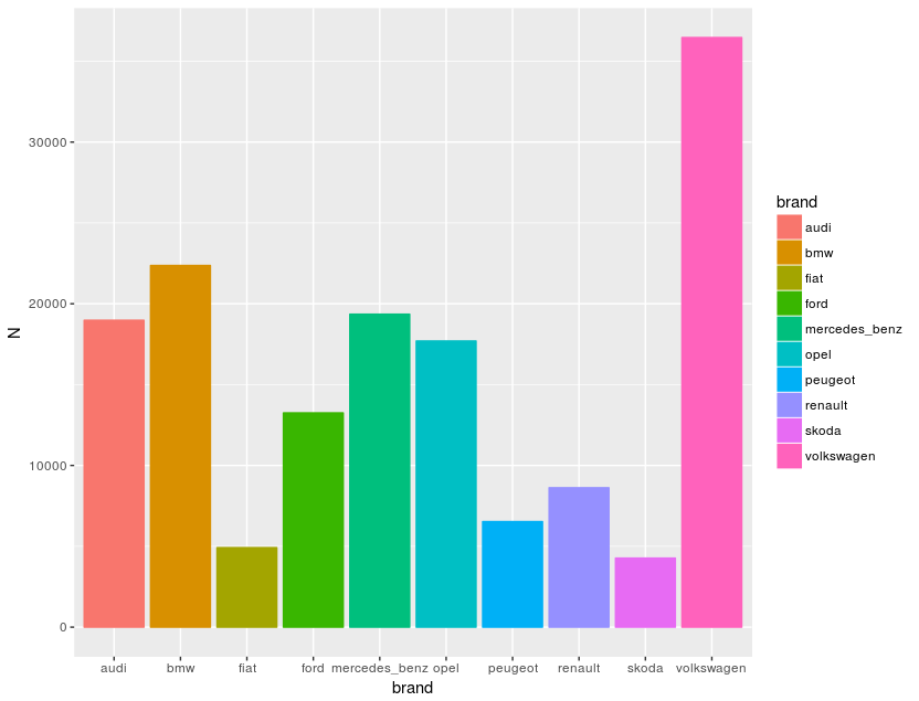
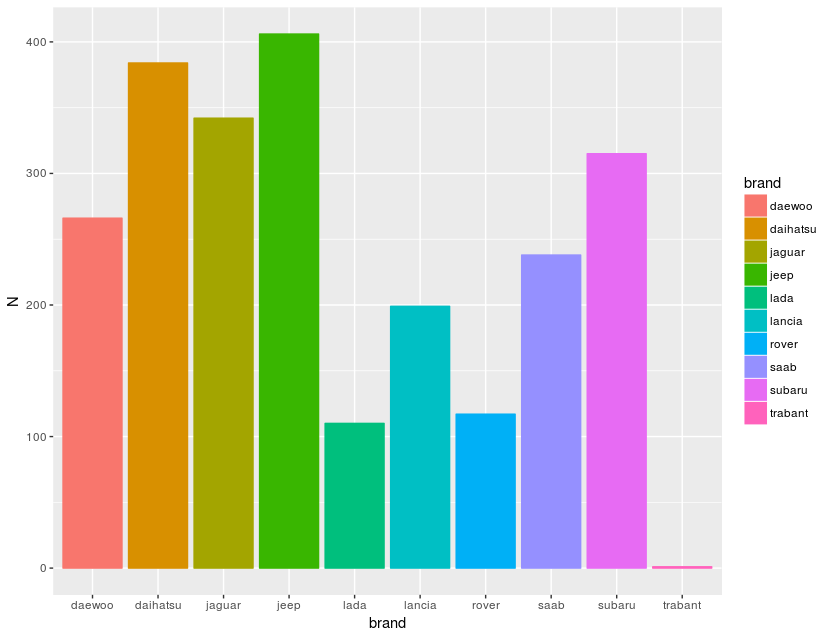
得到的結論是 volkswagen > bmw > audi > benz > opel,業務先生大概可信度是70%,再看看後段班,確實另人長知識了,Google trabant 是一個停產20多年車廠,原來上世紀還有這款車:
** 價格趨勢 **
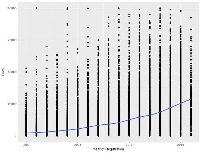
在原 Dataset 中他們展示了 yearOfRegistration 與 price 的迴歸模型。那我也來作個標準的 R 準本線性模型, :
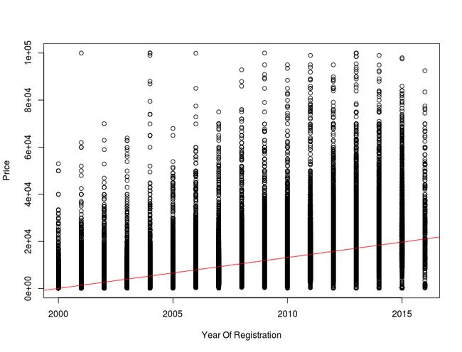
好吧,標準的 ploter 是比較難看點,那我們還是用 ggplot 來看趨勢線:
# year of registration and prices
ggplot(autos, aes(x = yearOfRegistration, y = price)) +
  geom_point() + geom_smooth()  +  ylim(c(0,100000)) +
  xlab("Year of Registration") + ylab("Price")
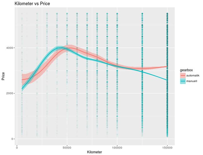
然後再來看每一種組合的趨勢線,這裡就展示其一種組合,按正規研究方法是要去計算各組合的 MSE(mean squared error)來取得最好的預測結果,但在這不作那麼嚴謹的方法學:
ggplot(autos, aes(x = kilometer, y = price, fill = gearbox, colour = gearbox)) + geom_point(alpha = 0.01) +
geom_smooth() + ylim(c(0,median(autos$price))) + ggtitle("Kilometer vs Price") +
xlab("Kilometer") + ylab("Price")
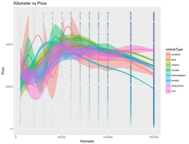
ggplot(autos, aes(x = kilometer, y = price, fill = vehicleType, colour = vehicleType)) + geom_point(alpha = 0.01) +
geom_smooth() + ylim(c(0,median(autos$price))) + ggtitle("Kilometer vs Price") +
xlab("Kilometer") + ylab("Price")
** 迴歸 **
在這裡我採用了 Tensorflow 的線性迴歸,而在前置處理前,記得要將類別(category)資料轉換為數字,可使用 sklearn.preprocessing.LabelEncoder:
for f in en_features:
    le = preprocessing.LabelEncoder()
    le.fit(list(set(autos[f])))
    autos[f] = le.transform(autos[f])
而我將預測值-price 取對數來將其 MSE 縮小到 0.05770393558656561,不過我覺得這有待商確,取樣的預測跟實際值如下:
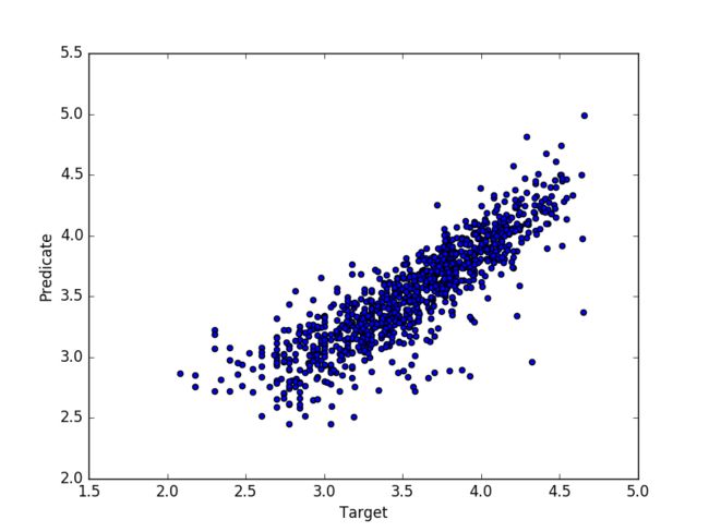
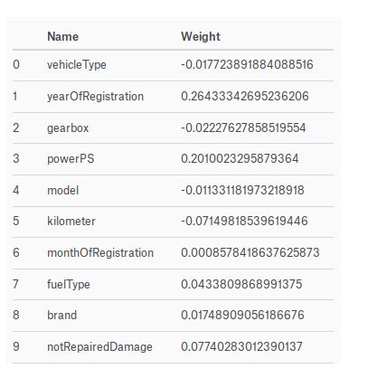
但我認為其實這個預測重要的還是在各因子對實際 Price 的影響程度,而不是結果值,所以輸出權重值來參考,但可能也不是每個人都認同這個想法,從這個表可看到影響二手車的價格主要為 ** Year Of Registration, PowerPS, Not Repaired Damage **,所以如果要買賣二手車可以參考看看:
詳細的程式可以在我發表在 Kaggle 的程式:TensorFlow LinearRegressor