k-medoids 算法思想
自wikipedia
The k-medoids algorithm is a clustering algorithm related to the k-means algorithm and the medoidshift algorithm. Both the k-means and k-medoids algorithms are partitional (breaking the dataset up into groups) and both attempt to minimize the distance between points labeled to be in a cluster and a point designated as the center of that cluster. In contrast to the k-means algorithm, k-medoids chooses datapoints as centers (medoids or exemplars) and works with an arbitrary matrix of distances between datapoints instead of ![]() . This method was proposed in 1987[1] for the work with
. This method was proposed in 1987[1] for the work with ![]() norm and other distances.
norm and other distances.
k-medoid is a classical partitioning technique of clustering that clusters the data set of n objects into k clusters known a priori. A useful tool for determining k is the silhouette.
It is more robust to noise and outliers as compared to k-means because it minimizes a sum of pairwise dissimilarities instead of a sum of squared Euclidean distances.
A medoid can be defined as the object of a cluster, whose average dissimilarity to all the objects in the cluster is minimal i.e. it is a most centrally located point in the cluster.
The most common realisation of k-medoid clustering is the Partitioning Around Medoids (PAM) algorithm and is as follows:[2]
- Initialize: randomly select k of the n data points as the medoids
- Associate each data point to the closest medoid. ("closest" here is defined using any valid distance metric, most commonly Euclidean distance, Manhattan distance orMinkowski distance)
- For each medoid m
- For each non-medoid data point o
- Swap m and o and compute the total cost of the configuration
- For each non-medoid data point o
- Select the configuration with the lowest cost.
- repeat steps 2 to 4 until there is no change in the medoid.
Contents[hide]
|
[edit]Demonstration of PAM
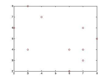
Cluster the following data set of ten objects into two clusters i.e. k = 2.
Consider a data set of ten objects as follows:
| X1 | 2 | 6 |
| X2 | 3 | 4 |
| X3 | 3 | 8 |
| X4 | 4 | 7 |
| X5 | 6 | 2 |
| X6 | 6 | 4 |
| X7 | 7 | 3 |
| X8 | 7 | 4 |
| X9 | 8 | 5 |
| X10 | 7 | 6 |
[edit]Step 1
Initialize k centers.
Let us assume c1 = (3,4) and c2 = (7,4)
So here c1 and c2 are selected as medoids.
Calculate distance so as to associate each data object to its nearest medoid. Cost is calculated using Manhattan distance (Minkowski distance metric with r = 1). Costs to the nearest medoid are shown bold in the table.
| i | c1 | Data objects (Xi) | Cost (distance) | ||
| 1 | 3 | 4 | 2 | 6 | 3 |
| 3 | 3 | 4 | 3 | 8 | 4 |
| 4 | 3 | 4 | 4 | 7 | 4 |
| 5 | 3 | 4 | 6 | 2 | 5 |
| 6 | 3 | 4 | 6 | 4 | 3 |
| 7 | 3 | 4 | 7 | 3 | 5 |
| 9 | 3 | 4 | 8 | 5 | 6 |
| 10 | 3 | 4 | 7 | 6 | 6 |
| i | c2 | Data objects (Xi) | Cost (distance) | ||
| 1 | 7 | 4 | 2 | 6 | 7 |
| 3 | 7 | 4 | 3 | 8 | 8 |
| 4 | 7 | 4 | 4 | 7 | 6 |
| 5 | 7 | 4 | 6 | 2 | 3 |
| 6 | 7 | 4 | 6 | 4 | 1 |
| 7 | 7 | 4 | 7 | 3 | 1 |
| 9 | 7 | 4 | 8 | 5 | 2 |
| 10 | 7 | 4 | 7 | 6 | 2 |
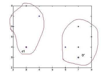
Then the clusters become:
Cluster1 = {(3,4)(2,6)(3,8)(4,7)}
Cluster2 = {(7,4)(6,2)(6,4)(7,3)(8,5)(7,6)}
Since the points (2,6) (3,8) and (4,7) are closer to c1 hence they form one cluster whilst remaining points form another cluster.
So the total cost involved is 20.
Where cost between any two points is found using formula
where x is any data object, c is the medoid, and d is the dimension of the object which in this case is 2.
Total cost is the summation of the cost of data object from its medoid in its cluster so here:
[edit]Step 2
Select one of the nonmedoids O′
Let us assume O′ = (7,3)
So now the medoids are c1(3,4) and O′(7,3)
If c1 and O′ are new medoids, calculate the total cost involved
By using the formula in the step 1
| i | c1 | Data objects (Xi) | Cost (distance) | ||
| 1 | 3 | 4 | 2 | 6 | 3 |
| 3 | 3 | 4 | 3 | 8 | 4 |
| 4 | 3 | 4 | 4 | 7 | 4 |
| 5 | 3 | 4 | 6 | 2 | 5 |
| 6 | 3 | 4 | 6 | 4 | 3 |
| 7 | 3 | 4 | 7 | 4 | 4 |
| 9 | 3 | 4 | 8 | 5 | 6 |
| 10 | 3 | 4 | 7 | 6 | 4 |
| i | O′ | Data objects (Xi) | Cost (distance) | ||
| 1 | 7 | 3 | 2 | 6 | 8 |
| 3 | 7 | 3 | 3 | 8 | 9 |
| 4 | 7 | 3 | 4 | 7 | 7 |
| 5 | 7 | 3 | 6 | 2 | 2 |
| 6 | 7 | 3 | 6 | 4 | 2 |
| 7 | 7 | 3 | 7 | 4 | 1 |
| 9 | 7 | 3 | 8 | 5 | 3 |
| 10 | 7 | 3 | 7 | 6 | 3 |
So cost of swapping medoid from c2 to O′ is
So moving to O′ would be a bad idea, so the previous choice was good. So we try other nonmedoids and found that our first choice was the best. So the configuration does not change and algorithm terminates here (i.e. there is no change in the medoids).
It may happen some data points may shift from one cluster to another cluster depending upon their closeness to medoid.
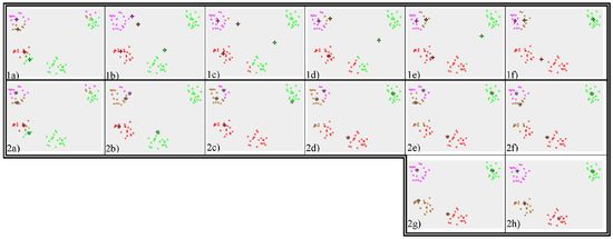
In some standard situations, k-medoids demonstrate better performance than k-means. An example is presented in Fig. 2. The most time-consuming part of the k-medoids algorithm is the calculation of the distance matrix between objects. Recently, a new algorithm for K-medoids clustering is proposed which runs not worse than the k-means. This algorithm calculates the distance matrix once and uses it for finding new medoids at every iterative step.[4] A comparative study of K-means and k-medoids algorithms was performed for normal and for uniform distributions of data points.[5] It was demonstrated that in the asymptotic of large data sets the k-medoids algorithm takes less time.


