作者:周纵苇
微博:@MrGiovanni
邮箱:[email protected]
References
[1.1] 2017 Data Science Bowl, Predicting Lung Cancer: 2nd Place Solution Write-up, Daniel Hammack and Julian de Wit
[1.2] Predicting lung cancer
[1.3] technical writeup: dsb_2017_daniel_hammack.pdf
Codes
[2.1] dhammack/DSB2017 on Github
>> Data Normalization - Unify the Resolution and Mapping
Sample the scans to a resolution of 1 mm = 1 pixel. [1.1]
Note: This step is important since different CT machines give different resolution especially in Z axis, named spacing.
Each scan is rescaled to lie between 0 and 1 with -1000 (air) mapping to 0 and +400 (bone) mapping to 1. [1.3]
Note: What about the HU larger than 400? Treat as water (0)?
Note: They only apply mapping into [0,1] without -mean and /std? (Z-score)
>> External Data
LIDC-IDRI (has malignancy labels!!! and radiologist descriptions!) and LUNA16
The properties that I chose to use were (sorted by importance): [1.1]
- nodule malignancy
- nodule diameter (size in mm, bigger is usually more cancerous)
- nodule spiculation (how "stringy" a nodule is - more is worse)
- nodule lobulation (how "bubbly" a nodule is - more is worse)
calcification (钙化)sphericity (对称性)
Note: Segmentation information (physical size)
>> Regular Solution
- 64mm^3 cube for training, and test on every location (slice window likely), then get a "nodule probabilities" map of
300x300x400mmwhole scan. [1.1]
Note: 是否统计过LUNA里面nodule的尺寸分布情况,64mm^3的patch size是怎么得出来的?
Note: 我比较好奇这个3D的分类器的cross validation的performance... 怎么看起来这么容易呢 :-) - Aggregate these with simple stats like max, stdev, and the location of the max probability prediction... get a feature vector. [1.1]
- Logistic Regression to forecast the diagnosis. Trained and validated on the Kaggle DSB dataset. [1.1]
>> Brain Storm
- Instead of predicting probability of a nodule existing, predict the size of the nodule (nodule size is in the LUNA dataset). [1.1]
Wonder: How to train the model using size ground truth?
Note: It will definite improve using size instead of binary label. 如果size的预测值可以更显著的分开,比如加上2的size次幂,让size起到更大的作用可能会更好,但是也说不准,不一定size大的malignancy就大...
- Add data augmentation [1.1]
- Improved model architecture (mainly added more batch norm) [1.1]
Note: 看来Batch Norm果然是很实用的方法,不知道这里的model用的是什么?ResNet or VGG or others? 调整网络的深度可能起到的效果并不显著?
- After discovering their existence, add LIDC features (malignancy especially) [1.1]
Note: 不知道add的LIDC features在后续的Kaggle DSB dataset上面怎么用?
- Improved aggregation of chunk predictions [1.1]
- Improving final diagnosis model (Logistic Regression + Extra Trees) [1.1]
Note: 应该来说Random Forest是比较promising的传统分类器
>> Data Augmentation - Use 3D data augmentation
Normal computer vision datasets have 10k-10m images.
Mirroring is an example of a "lossless transformation" of an image. [1.1]
Note: 对于自然图像可能是没有什么影响,但是医学影像不一定,很可能镜像一下就不符合实际情况了,比如心脏,只可能出现在左边。
There are 48 unique lossless permutation of 3D images as opposed to only 8 for 2D images. The studies is called Group Theory. [1.1]
You can show an image to the model a bunch of times with different random transformations and average the predictions it gives you. This is called “test time augmentation” and is another trick I used to improve performance. [1.1]
Note: In our paper, Fine-Tuning Convolutional Neural Networks for Biomedical Image Analysis: Actively and Incrementally, we prefer to use majority predictions instead of average.
We exploit all the symmetries of 3D space and use both lossless and lossy augmentation. We use random rotations by 90◦increments, random transpositions, random zooming by small amounts, random reordering of axes, and random arbitrary rotations by small degrees (-10 to 10). [1.3]
**Check: 需要弄清楚他们到底用了什么Data Augmentation的方法,是不是用的Keras自带的ImageDataGenerator. **
The lossy data augmentation is quite computationally expensive so we did not apply those transformations in real time during training but had a parallel process continually rebuild different versions of the training set. The training set was reloaded with a newly augmented version after every few epochs. [1.3]
Check: The training set was reloaded with a newly augmented version after every few epochs: 我一直都想做这样实时Augmentation,不知道他们是怎么实现的?
>> About Training a Model
One of the nice things about the architecture that I used was that the model can be trained on any sized input (of at least 32x32x32 in size). This is because the last pooling layer in my model is a global max pooling layer which returns a fixed length output no matter the input size. Because of this, I am able to use ‘curriculum learning’ to speed up model training. [1.1]
Note: Actually I don't really follow the idea here... What's the mean by "the last pooling layer is global max pooling layer"? How can I apply it on my experiment?
Curriculum learning is a technique in machine learning where a model is first trained on simpler or easier samples before gradually progressing to harder samples (much like human learning). Since the 32x32x32 chunks are easier/faster to train on than 64x64x64, I train the models on size 32 chunks first and then 64 chunks after. [1.1]
Note: He assumes that small size of chunks are easier samples for training.
Note: Active Learning requires hard samples even at the beginning, which is opposed to Curriculum Learning. Injecting randomness is somehow weakening Active Learning and strengthening Curriculum Learning at the beginning.
Because our model uses a global max pooling layer, it can process any input of size 32 mm^3 or larger. Thus because images of size 32 mm^3 are 8x smaller than 64 mm^3, we trained our model first on inputs of this size for about 2000 parameter updates with a batch size of 128. Then we increased the input size to 64 mm^3 and trained for 6000 parameter updates with a batch size of 64. [1.3]
The first 25 (out of 30 total) epochs were trained with a random choice of 75% of the nodules (different for each model) and the last 5 were with the full training set. [1.3]
The learning rate started at 0.1 and was decreased stepwise every few epochs. The last few epochs of training use a very low learning rate of 3e-5 which we found to help. [1.3]
How to tune the network (这是个很实用的问题,也是很花时间的,我不知道有什么好的方法来调参数,现在普遍用的就是用Cross Validation的效果来调参... 确实主要会去调这几个东西):
- the subset of data the model was trained on (random 75%) [1.1]
- activation function (relu/leakly relu mostly) [1.1]
- loss function and weights on loss objectives [1.1]
- training length/schedule [1.1]
- model layer sizes [1.1]
- model connection/branching structure [1.1]
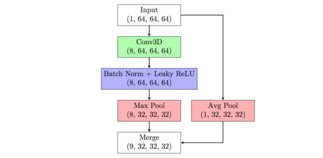
网络结构示意. "4x" refers to four parallel copies of that layer - one for each output in our multi output model [1.3]
Note: 4x的意思是四个并列的结构,它们的output分别是diam, lob, spic, malig。作者相当于把它们放到一起训练了,而不是单独去训练四个网络,实现的代码[2.1 build_nodule_describer_v34.py]如下:
... ...
#from here let's branch and predict different things
x3_ident = AveragePooling2D()(x2_ident)

x3_diam = conv_block(x2_merged,36,activation='crelu',init=looks_linear_init) #outputs 25 + 16 ch = 41
x3_lob = conv_block(x2_merged,36,activation='crelu',init=looks_linear_init) #outputs 25 + 16 ch = 41
x3_spic = conv_block(x2_merged,36,activation='crelu',init=looks_linear_init) #outputs 25 + 16 ch = 41
x3_malig = conv_block(x2_merged,36,activation='crelu',init=looks_linear_init) #outputs 25 + 16 ch = 41

x3_diam_merged = merge([x3_diam,x3_ident],mode='concat', concat_axis=1)
x3_lob_merged = merge([x3_lob,x3_ident],mode='concat', concat_axis=1)
x3_spic_merged = merge([x3_spic,x3_ident],mode='concat', concat_axis=1)
x3_malig_merged = merge([x3_malig,x3_ident],mode='concat', concat_axis=1)

... ...
model = Model(input=xin,output=[xout_diam, xout_lob, xout_spic, xout_malig])
Check: Don't understand "global max pooling"
| Layer Number | Name | Output Shape |
|---|---|---|
| 0 | Input | (1,64,64,64) |
| 1 | conv block | (8,32,32,32) |
| 2 | merge w/downsampled input | (9,32,32,32) |
| 3 | conv block | (24,16,16,16) |
| 4 | merge w/downsampled input | (25,16,16,16) |
| 5 | conv block | (48,8,8,8) |
| 6 | merge w/downsampled input | (49,8,8,8) |
| 7 | conv block | (64,4,4,4) |
| 8 | merge w/downsampled input | (65,4,4,4) |
| 9 | 4x conv block | 4 x (65,2,2,2) |
| 10 | 4x global max pooling | 4 x (65) |
| 11 | linear + softplus | 4 x (1) |
Structure of a conv block [1.3]:
Conv Block的实现函数[2.1 build_nodule_describer_v34.py]
def conv_block(x_input, num_filters, pool=True, activation='relu', init='orthogonal'):
    x1 = Convolution2D(num_filters,3,3,border_mode='same',W_regularizer=l2(1e-4),init=init)(x_input)
    x1 = BatchNormalization(axis=1,momentum=0.995)(x1)
    x1 = Lambda(leakyCReLU, output_shape=leakyCReLUShape)(x1)
    x1 = MaxPooling2D()(x1)
    return x_1
Note: 这个网络结构我没有用过,好像和VGG,GoogleNet不太一样。
The details of Deep Neural Network setup:
The input to all our neural network models are 64 mm^3 regions of the CT scan. [1.3]
Models consist of 5 "conv blocks", followed by global max pooling and a nonnegative regression layer with a softplus activation. To help the model capture information at different scales the original input is downsampled and fed into each layer of the model, not just the first. [1.3]
Softplus activation is used because the targets for the model were non-negative (we also used scaled sigmoid in some models). [1.3]
Note: softplus is f(x)=ln[1+exp(x)]
Most models were trained with a MSE objective but some were trained with MAE and some with log loss. Models were trained with the NAdam optimizer (Adam with Nesterov momentum) from the Keras package. [1.3]
Note: mean_squared_error (MSE), model.compile(loss='mean_squared_error')
Note: Nesterov Adam optimizer. keras.optimizers.Nadam(lr=0.002, beta_1=0.9, beta_2=0.999, epsilon=1e-08, schedule_decay=0.004)
We use 3D convolutions with filter size 3x3x3 everywhere, and pooling is always 2x2x2 with stride 2. [1.3]
Note: I got confused which size of convolutional kernel is most useful... It seems to me many researchers prefer 3x3x3, but some researchers also use 1x1x1. 我记得Stanford University的CS231n 2017的讲义上面有提到说1x1x1的卷积核最好。
Batch normalization is used after each convolution and max pooling is used for downsampling after batch norm. [1.3]
Most of our models use the leaky rectifier activation function. [1.3]
Note: 我一般都用的是ReLU,以后可以尝试一下Leaky ReLU。
Models were typically built on 75% of the data and validated on the other 25%. The models that are used for detecting abnormalities were trained with 90% non-nodules and 10% nodules, and the models for predicting nodule attributes had the opposite distribution. [1.3]
Check: 不知道他们在调试网络的时候有没有用到x-Fold Cross Validation,因为很费时间,我需要看代码才能知道在实际应用中他们是怎么划分训练集和测试集的。
>> Ensembling, to combine multiple models predictions together
Ultimately their solution combines 17 3D convolutional neural network models and consists of two ensembles. [1.3]
Note: 不同的组合有很多,作者report的是各种组合效果都接近,但是在实际的操作过程中,并不会这么顺利的,而且我遇到过就算用的相同的set up,最后converge的model performance都会有比较大的差别。很多团队会把大多数的时间和精力花在这个上面,但是我认为是比较浪费的,因为这个过程很费时间,又不怎么需要动脑子,一般的结果就是在deadline来之前一直在调参,当回顾比赛的全过程的时候发现真正novelty activity的时间并不多。
Note: 我当时做的时候也是训练了好几个models, with different settings, parameters, data, and objectives, 但是我都是分别测试使用的,并没有想到把它们的结果ensemble起来。
>> Pipeline
- Normalize scan [1.1]
- Discard regions which appear normal or are irrelevant [1.1]
Note: Remove irrelative part - require 100% sensitivity and may generate many false positives, that's fine. 关于这个requirement,我们最近是在研究如何在保证Sensitivity的前提下去push specificity,也就是说,最后的AUC可以不好,但是ROC曲线是要往High Sensitivity方向去靠。在临床上这是一个很重要的问题。So this dataset is potentially great application for paper.
Check: 不同的CT scan最后留下来训练的区域大小数目是不一样的,而且我觉得这个步骤用的可能是传统的方法,不需要训练的那种,在testing的时候,也会自动的剔除掉irrelative的部分。因此Nodule Attribute Predictions的Feature就只能是统计上的一些指标了。我们在做的时候是Nodule Detection,实质上是需要训练网络的,对于这部分我需要进一步的研究,到底是用先验知识来设计Feature,还是直接用Deep Learning end2end。 - Predict nodule attributes (e.g. size, malignancy) in abnormal regions using a big ensemble of models [1.1]
- Combine nodule attribute predictions into a diagnosis (probability of cancer) [1.1]
>> 根据Prediction Map来设计特征
他们所使用的18个特征 [1.3]
- max malignancy/spiculation/lobulation/diameter (4)
- stdev malignancy/spiculation/lobulation/diameter (4)
- location of most malignant nodule (3, one for each dimension in the scan)
Note: 每个3D scan只挑出来一个nodule,malignancy最大,也就说即便有多个malignant,也只取maximum。前提是malignancy分类器确实很不错。 - stdev of nodule locations in each dimension (3)
- nodule clustering features (4) - running a clustering algorithm on the nodule locations
Note: 这部分很有意思啦,我不知道在remove掉很多irrelative parts之后,留下来坑坑洼洼的ROI,他们是怎么计算Nodule的直径的... 如果可以算直径的话说明那个训练器的效果确实很好。
Note: 然后还有spiculation这种指标该怎么算,我的预判是网络的输出应该不会特别的理想啊,要想得到清晰的轮廓有这么容易吗?不应该是prediction map想云一样模模糊糊的吗,如此算出来的spiculation真的可靠吗?
Check: 不知道这里用的是分类模型CNN...还是分割模型UNet/FCN... 我需要去看他们的code才能弄清楚。
Also one additional feature was added late - the output of Julian's mass detector model. It predicts the amount of "abnormal mass" in the lungs of a patient. [1.3]

