02_行销（Marketing）里用逻辑回归来找寻顾客参与度后面的原因

进行市场营销活动时，查看和分析的重要指标之一是客户参与营销活动。例如，在电子邮件营销中，可以通过客户打开或忽略了多少营销电子邮件来衡量客户参与度。客户参与度也可以通过单个客户的网站访问量来衡量。成功的市场营销活动将吸引客户大量参与，而无效的市场营销活动不仅会降低客户的参与度，还会对业务产生负面影响。客户可能会将来自你公司的电子邮件标记为垃圾邮件，或者取消订阅您的邮件列表。为了理解什么会影响客户参与度，在本章中，我们将讨论如何使用解释性分析（更具体地说，是回归分析）。我们将简要介绍解释性分析的定义，什么是回归分析以及如何使用逻辑回归模型进行解释性分析。然后，我们将介绍如何使用statsmodels包在Python中构建和解释回归分析结果。在这篇文章里我仍会用一个Kaggle的数据集来演示。数据来源于 WA_Fn-UseC_-Marketing-Customer-Value-Analysis.csv。

Logistic回归是一种回归分析，当输出变量为binary时（对于阳性结果为一个，对于阴性结果为零），将使用回归分析。像任何其他线性回归模型一样，逻辑回归模型从特征变量的线性组合估计输出。唯一的区别是模型估计的值。与其他线性回归模型不同，逻辑回归模型估计事件的对数几率，换句话说，估计正事件和负事件概率之间的对数比

左边的比率是成功的几率，它表示成功的概率与失败的概率之间的比率。 Logistic回归模型输出只是logit的倒数，范围从零到一。在本章中，我们将使用回归分析来了解推动客户参与度的因素，而输出变量将是客户是否响应了营销电话。因此，逻辑回归非常适合这种情况，因为输出是一个可以采用两个值的二变量：已响应与未响应。下面我们用Kaggle的数据做一个逻辑回归来看怎么做统计分析。

# This Python 3 environment comes with many helpful analytics libraries installed
# It is defined by the kaggle/python Docker image: https://github.com/kaggle/docker-python
# For example, here's several helpful packages to load

import numpy as np # linear algebra
import pandas as pd # data processing, CSV file I/O (e.g. pd.read_csv)

# Input data files are available in the read-only "../input/" directory
# For example, running this (by clicking run or pressing Shift+Enter) will list all files under the input directory

import os
for dirname, _, filenames in os.walk('/kaggle/input'):
    for filename in filenames:
        print(os.path.join(dirname, filename))

# You can write up to 5GB to the current directory (/kaggle/working/) that gets preserved as output when you create a version using "Save & Run All" 
# You can also write temporary files to /kaggle/temp/, but they won't be saved outside of the current session

/kaggle/input/ibm-watson-marketing-customer-value-data/WA_Fn-UseC_-Marketing-Customer-Value-Analysis.csv

Load packages

import matplotlib.pyplot as plt
import pandas as pd
import statsmodels.formula.api as sm
import statsmodels.api as sm
%matplotlib inline

df = pd.read_csv('../input/ibm-watson-marketing-customer-value-data/WA_Fn-UseC_-Marketing-Customer-Value-Analysis.csv')
df.head(3)

	Customer	State	Customer Lifetime Value	Response	Coverage	Education	Effective To Date	EmploymentStatus	Gender	Income	...	Months Since Policy Inception	Number of Open Complaints	Number of Policies	Policy Type	Policy	Renew Offer Type	Sales Channel	Total Claim Amount	Vehicle Class	Vehicle Size
0	BU79786	Washington	2763.519279	No	Basic	Bachelor	2/24/11	Employed	F	56274	...	5	0	1	Corporate Auto	Corporate L3	Offer1	Agent	384.811147	Two-Door Car	Medsize
1	QZ44356	Arizona	6979.535903	No	Extended	Bachelor	1/31/11	Unemployed	F	0	...	42	0	8	Personal Auto	Personal L3	Offer3	Agent	1131.464935	Four-Door Car	Medsize
2	AI49188	Nevada	12887.431650	No	Premium	Bachelor	2/19/11	Employed	F	48767	...	38	0	2	Personal Auto	Personal L3	Offer1	Agent	566.472247	Two-Door Car	Medsize

3 rows ?? 24 columns

Generate engage category

df['Engaged'] = df['Response'].apply(lambda x: 0 if x == 'No' else 1)
df.head(3)

	Customer	State	Customer Lifetime Value	Response	Coverage	Education	Effective To Date	EmploymentStatus	Gender	Income	...	Number of Open Complaints	Number of Policies	Policy Type	Policy	Renew Offer Type	Sales Channel	Total Claim Amount	Vehicle Class	Vehicle Size	Engaged
0	BU79786	Washington	2763.519279	No	Basic	Bachelor	2/24/11	Employed	F	56274	...	0	1	Corporate Auto	Corporate L3	Offer1	Agent	384.811147	Two-Door Car	Medsize	0
1	QZ44356	Arizona	6979.535903	No	Extended	Bachelor	1/31/11	Unemployed	F	0	...	0	8	Personal Auto	Personal L3	Offer3	Agent	1131.464935	Four-Door Car	Medsize	0
2	AI49188	Nevada	12887.431650	No	Premium	Bachelor	2/19/11	Employed	F	48767	...	0	2	Personal Auto	Personal L3	Offer1	Agent	566.472247	Two-Door Car	Medsize	0

3 rows ?? 25 columns

Engagement Rate

engagement_rate_df = pd.DataFrame(
    df.groupby('Engaged').count()['Response'] / df.shape[0] * 100.0
)
engagement_rate_df.T

Engaged	0	1
Response	85.679877	14.320123

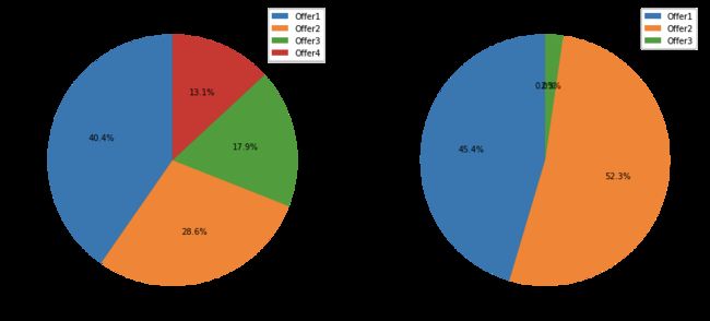
Engage By Renew Offer Type

engagement_by_offer_type_df = pd.pivot_table(
    df, values='Response', index='Renew Offer Type', columns='Engaged', aggfunc=len
).fillna(0.0)

engagement_by_offer_type_df.columns = ['Not Engaged', 'Engaged']
engagement_by_offer_type_df

	Not Engaged	Engaged
Renew Offer Type
Offer1	3158.0	594.0
Offer2	2242.0	684.0
Offer3	1402.0	30.0
Offer4	1024.0	0.0

engagement_by_offer_type_df.plot(
    kind='pie',
    figsize=(15, 7),
    startangle=90,
    subplots=True,
    autopct=lambda x: '%0.1f%%' % x
)

plt.show()

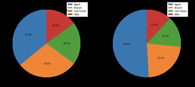
Engage By Sales Channel

engagement_by_sales_channel_df = pd.pivot_table(
    df, values='Response', index='Sales Channel', columns='Engaged', aggfunc=len
).fillna(0.0)

engagement_by_sales_channel_df.columns = ['Not Engaged', 'Engaged']
engagement_by_sales_channel_df

	Not Engaged	Engaged
Sales Channel
Agent	2811	666
Branch	2273	294
Call Center	1573	192
Web	1169	156

engagement_by_sales_channel_df.plot(
    kind='pie',
    figsize=(15, 7),
    startangle=90,
    subplots=True,
    autopct=lambda x: '%0.1f%%' % x
)

plt.show()

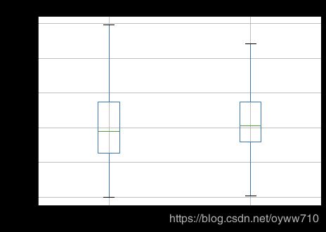
Total Claim Amount Distributions

ax = df[['Engaged', 'Total Claim Amount']].boxplot(
    by='Engaged',
    showfliers=False,  ## this will help remove outlier
    figsize=(7,5)
)

ax.set_xlabel('Engaged')
ax.set_ylabel('Total Claim Amount')
ax.set_title('Total Claim Amount Distributions by Enagements')

plt.suptitle("")
plt.show()

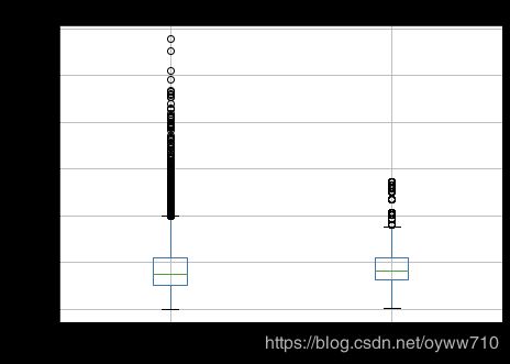
If we don’t want to remove outliers

ax = df[['Engaged', 'Total Claim Amount']].boxplot(
    by='Engaged',
    showfliers=True,
    figsize=(7,5)
)

ax.set_xlabel('Engaged')
ax.set_ylabel('Total Claim Amount')
ax.set_title('Total Claim Amount Distributions by Enagements')

plt.suptitle("")
plt.show()

Income Distributions

ax = df[['Engaged', 'Income']].boxplot(
    by='Engaged',
    showfliers=True,
    figsize=(7,5)
)

ax.set_xlabel('Engaged')
ax.set_xlabel('Income')
ax.set_title('Income Distributions by Enagements')

plt.suptitle("")
plt.show()

df.groupby('Engaged').describe()['Income'].T

Engaged	0	1
count	7826.000000	1308.000000
mean	37509.190008	38544.027523
std	30752.259099	28043.637944
min	0.000000	0.000000
25%	0.000000	18495.000000
50%	34091.000000	32234.000000
75%	62454.250000	60880.000000
max	99981.000000	99845.000000

Regression using different features

continuous_vars = [
    'Customer Lifetime Value', 'Income', 'Monthly Premium Auto', 
    'Months Since Last Claim', 'Months Since Policy Inception', 
    'Number of Open Complaints', 'Number of Policies', 
    'Total Claim Amount'
]

df['Engaged']

0       0
1       0
2       0
3       0
4       0
       ..
9129    0
9130    1
9131    0
9132    0
9133    0
Name: Engaged, Length: 9134, dtype: int64

logit = sm.Logit(
    df['Engaged'], 
    df[continuous_vars]
)

logit_fit = logit.fit()

Optimization terminated successfully.
         Current function value: 0.421189
         Iterations 6

logit_fit.summary()

Logit Regression Results

Dep. Variable:	Engaged	No. Observations:	9134
Model:	Logit	Df Residuals:	9126
Method:	MLE	Df Model:	7
Date:	Sun, 10 May 2020	Pseudo R-squ.:	-0.02546
Time:	16:48:28	Log-Likelihood:	-3847.1
converged:	True	LL-Null:	-3751.6
Covariance Type:	nonrobust	LLR p-value:	1.000

	coef	std err	z	P>|z|	[0.025	0.975]
Customer Lifetime Value	-6.741e-06	5.04e-06	-1.337	0.181	-1.66e-05	3.14e-06
Income	-2.857e-06	1.03e-06	-2.766	0.006	-4.88e-06	-8.33e-07
Monthly Premium Auto	-0.0084	0.001	-6.889	0.000	-0.011	-0.006
Months Since Last Claim	-0.0202	0.003	-7.238	0.000	-0.026	-0.015
Months Since Policy Inception	-0.0060	0.001	-6.148	0.000	-0.008	-0.004
Number of Open Complaints	-0.0829	0.034	-2.424	0.015	-0.150	-0.016
Number of Policies	-0.0810	0.013	-6.356	0.000	-0.106	-0.056
Total Claim Amount	0.0001	0.000	0.711	0.477	-0.000	0.000

Looking at this model output, we can see that Income, Monthly Premium Auto, Months Since Last Claim, Months Since Policy Inception, and Number of Policies variables have significant relationships with the output variable, Engaged. For example, Number of Policies variable is significant and is negatively correlated with Engaged. This suggests that the more policies that the customers have, the less likely they are to respond to marketing calls. As another example, the Months Since Last Claim variable is significant and is negatively correlated with the output variable, Engaged. This means that the longer it has been since the last claim, the less likely that the customer is going to respond to marketing calls.

Next we add categorical variables. There are several ways to deal with categorical variables

factorize

labels, levels = df['Education'].factorize()

labels

array([0, 0, 0, ..., 0, 1, 1])

levels

Index(['Bachelor', 'College', 'Master', 'High School or Below', 'Doctor'], dtype='object')

pandas’ Categorical variable series

categories = pd.Categorical(
    df['Education'], 
    categories=['High School or Below', 'Bachelor', 'College', 'Master', 'Doctor']
)

categories.categories

Index(['High School or Below', 'Bachelor', 'College', 'Master', 'Doctor'], dtype='object')

categories.codes

array([1, 1, 1, ..., 1, 2, 2], dtype=int8)

Dummy variables

pd.get_dummies(df['Education']).head(10)

	Bachelor	College	Doctor	High School or Below	Master
0	1	0	0	0	0
1	1	0	0	0	0
2	1	0	0	0	0
3	1	0	0	0	0
4	1	0	0	0	0
5	1	0	0	0	0
6	0	1	0	0	0
7	0	0	0	0	1
8	1	0	0	0	0
9	0	1	0	0	0

gender_values, gender_labels = df['Gender'].factorize()
df['GenderFactorized'] = gender_values
categories = pd.Categorical(
    df['Education'], 
    categories=['High School or Below', 'Bachelor', 'College', 'Master', 'Doctor']
)
df['EducationFactorized'] = categories.codes

logit = sm.Logit(
    df['Engaged'], 
    df[[
        'GenderFactorized',
        'EducationFactorized'
    ]]
)

logit_fit = logit.fit()

Optimization terminated successfully.
         Current function value: 0.493068
         Iterations 6

logit_fit.summary()

Logit Regression Results

Dep. Variable:	Engaged	No. Observations:	9134
Model:	Logit	Df Residuals:	9132
Method:	MLE	Df Model:	1
Date:	Sun, 10 May 2020	Pseudo R-squ.:	-0.2005
Time:	16:54:00	Log-Likelihood:	-4503.7
converged:	True	LL-Null:	-3751.6
Covariance Type:	nonrobust	LLR p-value:	1.000

	coef	std err	z	P>|z|	[0.025	0.975]
GenderFactorized	-1.1266	0.047	-24.116	0.000	-1.218	-1.035
EducationFactorized	-0.6256	0.021	-29.900	0.000	-0.667	-0.585

All together in logistic regression

logit = sm.Logit(
    df['Engaged'], 
    df[['Customer Lifetime Value',
        'Income',
        'Monthly Premium Auto',
        'Months Since Last Claim',
        'Months Since Policy Inception',
        'Number of Open Complaints',
        'Number of Policies',
        'Total Claim Amount',
        'GenderFactorized',
        'EducationFactorized'
    ]]
)

logit_fit = logit.fit()
logit_fit.summary()

Optimization terminated successfully.
         Current function value: 0.420810
         Iterations 6

Logit Regression Results

Dep. Variable:	Engaged	No. Observations:	9134
Model:	Logit	Df Residuals:	9124
Method:	MLE	Df Model:	9
Date:	Sun, 10 May 2020	Pseudo R-squ.:	-0.02454
Time:	16:54:33	Log-Likelihood:	-3843.7
converged:	True	LL-Null:	-3751.6
Covariance Type:	nonrobust	LLR p-value:	1.000

	coef	std err	z	P>|z|	[0.025	0.975]
Customer Lifetime Value	-6.909e-06	5.03e-06	-1.373	0.170	-1.68e-05	2.96e-06
Income	-2.59e-06	1.04e-06	-2.494	0.013	-4.63e-06	-5.55e-07
Monthly Premium Auto	-0.0081	0.001	-6.526	0.000	-0.011	-0.006
Months Since Last Claim	-0.0194	0.003	-6.858	0.000	-0.025	-0.014
Months Since Policy Inception	-0.0057	0.001	-5.827	0.000	-0.008	-0.004
Number of Open Complaints	-0.0813	0.034	-2.376	0.017	-0.148	-0.014
Number of Policies	-0.0781	0.013	-6.114	0.000	-0.103	-0.053
Total Claim Amount	0.0001	0.000	0.943	0.346	-0.000	0.000
GenderFactorized	-0.1500	0.058	-2.592	0.010	-0.263	-0.037
EducationFactorized	-0.0070	0.027	-0.264	0.792	-0.059	0.045

Let’s take a closer look at this output. The Income, Monthly Premium Auto, Months Since Last Claim,Months Since Policy Inception, Number of Open Complaints, Number of Policies, and GenderFactorized variable are significant at a 0.05 significance level, and all of them have negative relationships with the output variable, Engaged. Hence, the higher the income is, the less likely that the customer will be engaged with marketing calls. Similarly, the more policies that the customer has, the less likely that he or she will be engaged with marketing calls.

Lastly, male customers are less likely to engage with marketing calls than female customers, which we can see from looking at the coefficient of GenderFactorized. From looking at this regression analysis output, we can easily see the relationships between the input and output variables, and we can understand which attributes of customers are positively or negatively related to customer engagement with marketing calls