11_行销（Marketing）里为了制定更好的营销策略的A/B testing

A / B测试在各个行业的决策过程中都扮演着至关重要的角色。 A / B测试本质上是一种比较和测试两种不同业务策略的有效性和收益的方法。可以认为这是一个实验，其中在指定的时间段内测试了两个或多个变体，然后评估了实验结果以找到最有效的策略。在完全承诺使用单个选项之前运行A / B测试有助于企业摆脱决策过程中的猜测，并节省宝贵的资源，例如时间和资本，如果选择的策略不起作用，这些资源可能会被浪费。

在典型的A / B测试设置中，将创建和测试两个或多个版本的营销策略，以了解它们在实现营销目标方面的有效性。考虑一种情况，如果我们的目标是提高营销电子邮件的打开率。如果我们的假设是电子邮件B的打开率比电子邮件主题A高，那么我们将对这两个主题行进行A / B测试。我们将随机选择一半的用户并发送主题行为A的市场营销电子邮件。另一半随机选择的用户将收到主题行为B的电子邮件。运行此测试一段预定的时间（可能为一周） ，例如两周或一个月），或者直到预定数量的用户收到两种版本的电子邮件（至少有1,000名用户才能接收主题行的每种版本）。测试完成后，便可以分析和评估实验结果。分析结果时，需要检查两个版本的结果之间是否在统计上有显着差异。除了上述电子邮件主题行场景之外，A / B测试还可以应用于许多不同的营销领域。例如，可以对社交媒体上的广告进行A / B测试。我们可以使用两个或多个广告变体，然后进行A / B测试，以查看哪种变体更适合点击率或转化率。再举一个例子，可以使用A / B测试来测试网页上的产品推荐是否会提高购买率。如果构建了其他版本的产品推荐算法，则可以使用产品推荐算法的初始版本并将其公开给某些随机选择的用户，将第二种版本公开给其他随机选择的用户。我们可以收集A / B测试结果，并评估哪种版本的产品推荐算法可帮助我们带来更多收入。

从这些示例用例中可以看到，A / B测试在决策中起着重要作用。在完全致力于某个方案之前测试不同的方案时，它可以帮助我们节省精力，时间和资本，A / B测试还可以帮助我们消除猜测，并量化未来营销策略的绩效收益（或损失）。每当有想要重复的新营销理念时，我们都应考虑先运行A / B测试。

当运行A / B测试时，检验假设并寻找测试组之间的统计学差异非常重要。学生t检验或简单的t检验经常用于检验两次检验之间的差异是否具有统计学显着性。 t检验比较两个平均值，并检查它们是否彼此显着不同。t检验中有两个重要的统计数据：t值和p值。 t值衡量相对于数据变化的差异程度。 t值越大，两组之间的差异就越大。另一方面，p值衡量的是偶然发生结果的可能性。 p值越小，两组之间的统计差异就越大。

在该方程式中，M1和M2是组1和2的平均值。S1和S2是组1和2的标准偏差，N1和N2分别是组1和2中的样本数。

在统计中我们有零假设和替代假设的概念。一般而言，零假设是两组均无统计学差异。另一方面，另一种假设指出，两组显示出统计学上的显着差异。当t值大于阈值而p值小于阈值时，我们说我们可以拒绝原假设，并且两组显示出统计学上的显着差异。通常，将0.01或0.05用作测试统计显着性的p值阈值。如果p值小于0.05，则表明两组之间偶然发生差异的可能性小于5％。换句话说，这种差异极不可能是偶然的。

在这篇里，我们来run一个A/B测试。数据来自于WA_Fn-UseC_-Marketing-Campaign-Eff-UseC_-FastF.csv

Load the packages

%matplotlib inline
import matplotlib.pyplot as plt
import pandas as pd

Load Data

df = pd.read_csv('WA_Fn-UseC_-Marketing-Campaign-Eff-UseC_-FastF.csv')

df.shape

(548, 7)

df.head(3)

	MarketID	MarketSize	LocationID	AgeOfStore	Promotion	week	SalesInThousands
0	1	Medium	1	4	3	1	33.73
1	1	Medium	1	4	3	2	35.67
2	1	Medium	1	4	3	3	29.03

Data Analysis

Total Sales

df['SalesInThousands'].describe()

count    548.000000
mean      53.466204
std       16.755216
min       17.340000
25%       42.545000
50%       50.200000
75%       60.477500
max       99.650000
Name: SalesInThousands, dtype: float64

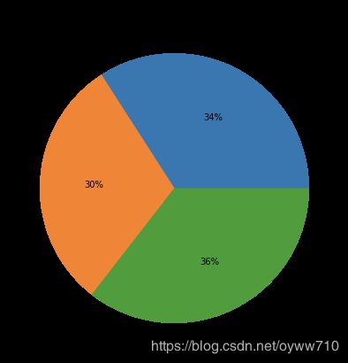
ax = df.groupby(
    'Promotion'
).sum()[
    'SalesInThousands'
].plot.pie(
    figsize=(7, 7),
    autopct='%1.0f%%'
)

ax.set_ylabel('')
ax.set_title('sales distribution across different promotions')

plt.show()

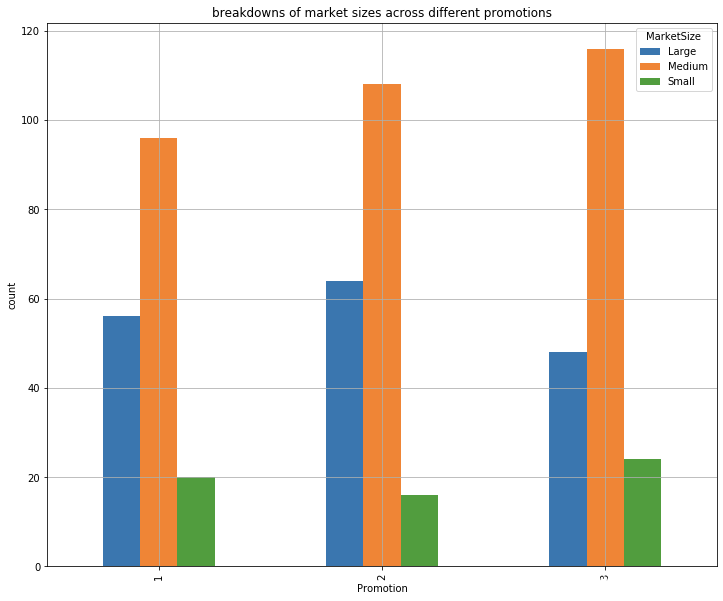
Market Size

df.groupby('MarketSize').count()['MarketID']

MarketSize
Large     168
Medium    320
Small      60
Name: MarketID, dtype: int64

ax = df.groupby([
    'Promotion', 'MarketSize'
]).count()[
    'MarketID'
].unstack(
    'MarketSize'
).plot(
    kind='bar',
    figsize=(12,10),
    grid=True,
)

ax.set_ylabel('count')
ax.set_title('breakdowns of market sizes across different promotions')

plt.show()

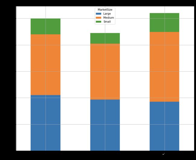
ax = df.groupby([
    'Promotion', 'MarketSize'
]).sum()[
    'SalesInThousands'
].unstack(
    'MarketSize'
).plot(
    kind='bar',
    figsize=(12,10),
    grid=True,
    stacked=True
)

ax.set_ylabel('Sales (in Thousands)')
ax.set_title('breakdowns of market sizes across different promotions')

plt.show()

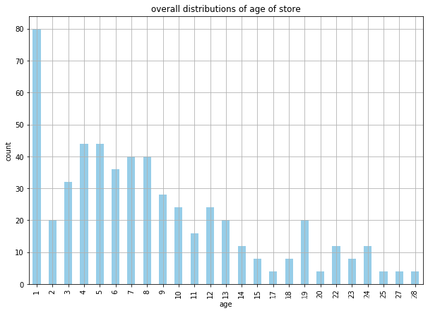
Store Age

df['AgeOfStore'].describe()

count    548.000000
mean       8.503650
std        6.638345
min        1.000000
25%        4.000000
50%        7.000000
75%       12.000000
max       28.000000
Name: AgeOfStore, dtype: float64

ax = df.groupby(
    'AgeOfStore'
).count()[
    'MarketID'
].plot(
    kind='bar', 
    color='skyblue',
    figsize=(10,7),
    grid=True
)

ax.set_xlabel('age')
ax.set_ylabel('count')
ax.set_title('overall distributions of age of store')

plt.show()

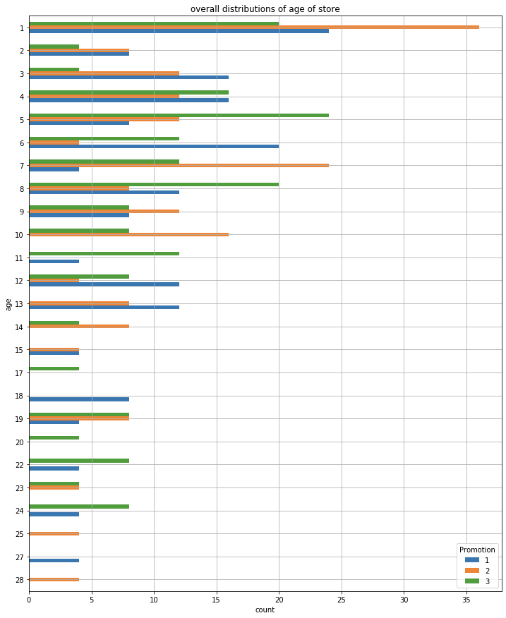
ax = df.groupby(
    ['AgeOfStore', 'Promotion']
).count()[
    'MarketID'
].unstack(
    'Promotion'
).iloc[::-1].plot(
    kind='barh', 
    figsize=(12,15),
    grid=True
)

ax.set_ylabel('age')
ax.set_xlabel('count')
ax.set_title('overall distributions of age of store')

plt.show()

df.groupby('Promotion').describe()['AgeOfStore']

	count	mean	std	min	25%	50%	75%	max
Promotion
1	172.0	8.279070	6.636160	1.0	3.0	6.0	12.0	27.0
2	188.0	7.978723	6.597648	1.0	3.0	7.0	10.0	28.0
3	188.0	9.234043	6.651646	1.0	5.0	8.0	12.0	24.0

Week Number

df.groupby('week').count()['MarketID']

week
1    137
2    137
3    137
4    137
Name: MarketID, dtype: int64

df.groupby(['Promotion', 'week']).count()['MarketID']

Promotion  week
1          1       43
           2       43
           3       43
           4       43
2          1       47
           2       47
           3       47
           4       47
3          1       47
           2       47
           3       47
           4       47
Name: MarketID, dtype: int64

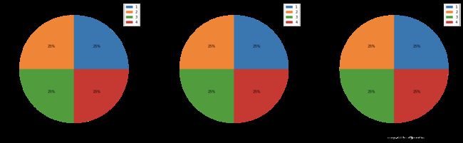
ax1, ax2, ax3 = df.groupby(
    ['week', 'Promotion']
).count()[
    'MarketID'
].unstack('Promotion').plot.pie(
    subplots=True,
    figsize=(24, 8),
    autopct='%1.0f%%'
)

ax1.set_ylabel('Promotion #1')
ax2.set_ylabel('Promotion #2')
ax3.set_ylabel('Promotion #3')

ax1.set_xlabel('distribution across different weeks')
ax2.set_xlabel('distribution across different weeks')
ax3.set_xlabel('distribution across different weeks')

plt.show()

Statistical Significance

import numpy as np
from scipy import stats

t-test

means = df.groupby('Promotion').mean()['SalesInThousands']
means

Promotion
1    58.099012
2    47.329415
3    55.364468
Name: SalesInThousands, dtype: float64

stds = df.groupby('Promotion').std()['SalesInThousands']
stds

Promotion
1    16.553782
2    15.108955
3    16.766231
Name: SalesInThousands, dtype: float64

ns = df.groupby('Promotion').count()['SalesInThousands']
ns

Promotion
1    172
2    188
3    188
Name: SalesInThousands, dtype: int64

Promotion 1 vs. 2

t_1_vs_2 = (
    means.iloc[0] - means.iloc[1]
)/ np.sqrt(
    (stds.iloc[0]**2/ns.iloc[0]) + (stds.iloc[1]**2/ns.iloc[1])
)

df_1_vs_1 = ns.iloc[0] + ns.iloc[1] - 2

p_1_vs_2 = (1 - stats.t.cdf(t_1_vs_2, df=df_1_vs_1))*2

t_1_vs_2

6.427528670907475

p_1_vs_2

4.143296816749853e-10

using scipy

t, p = stats.ttest_ind(
    df.loc[df['Promotion'] == 1, 'SalesInThousands'].values, 
    df.loc[df['Promotion'] == 2, 'SalesInThousands'].values, 
    equal_var=False
)

t

6.42752867090748

p

4.2903687179871785e-10

Promotion 1 vs 3

t_1_vs_3 = (
    means.iloc[0] - means.iloc[2]
)/ np.sqrt(
    (stds.iloc[0]**2/ns.iloc[0]) + (stds.iloc[2]**2/ns.iloc[2])
)

df_1_vs_3 = ns.iloc[0] + ns.iloc[1] - 2

p_1_vs_3 = (1 - stats.t.cdf(t_1_vs_3, df=df_1_vs_3))*2

t_1_vs_3

1.5560224307759116

p_1_vs_3

0.12058631176433687

using scipy

t, p = stats.ttest_ind(
    df.loc[df['Promotion'] == 1, 'SalesInThousands'].values, 
    df.loc[df['Promotion'] == 3, 'SalesInThousands'].values, 
    equal_var=False
)

t

1.5560224307758634

p

0.12059147742229478