自编码器图像去噪-pytorch实现

概念

自编码器的两个核心部分是编码器和解码器，它将输入数据压缩到一个潜在的空间中，然后再根据这个空间将数据进行重构得到最后的输出数据。整个架构都是采用神经网络构建，与普通的神经网络架构相似。

作用

1. 对图像去噪；
2. 对数据进行压缩降维；

数据

采用的数据是MNIST数据集，把数据集下载放在MNIST_data文件夹中，也可以先下载好数据集放在文件夹中。

网络构建

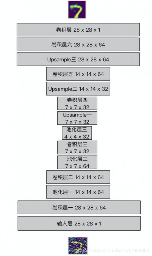
网络结构的编码器与普通的神经网络差不多，每一个卷积层的后面都有一个最大池化层来减少维度，直到想要的维度。网络结构的解码器是由一个窄的数据维度转换为一个宽的数据图像。例如：这里有一个由编码器输出的 4x4x8 的最大池化层，然后我们需要从解码器中得到一个 28x28x1的重构图像。这里本身是由编码器得到的 4x4x8，然后由卷积，岂不是变得更小，所以采用 Unsample(上采样)+卷积操作

网络机构示意图

输入层

input_x = tf.placeholder(tf.float32,  shape = (None,28,28,1), name = 'input_x')
target_x = tf.placeholder(tf.float32, shape =(None, 28,28,1), name='target_x')

编码器

conv_1 = tf.layers.conv2d(input_x, 64, (3,3), padding = 'same',activation=tf.nn.relu)
#shape=(28,28,64)
conv_1 = tf.layers.max_pooling2d(conv_1, (2,2), (2,2), padding = 'same')
#shape = (14,14,64)

conv_2 = tf.layers.conv2d(conv_1, 64, (3,3), padding = 'same', activation = tf.nn.relu)
#shape = (14,14,64)
conv_2 = tf.layers.max_pooling2d(conv_2, (2,2),(2,2), padding = 'same')
#shape = (7,7,64)

conv_3 = tf.layers.conv2d(conv_2,32,(3,3),padding ='same', activation=tf.nn.relu)
#shape = (7,7,32)
conv_3 = tf.layers.max_pooling2d(conv_3,(2,2),(2,2), padding = 'same')
#shape = (4,4,32)

解码器

# Decoder
conv_4 = tf.image.resize_nearest_neighbor(conv_3, (7,7))
#shape = (7,7,32)
conv_4 = tf.layers.conv2d(conv_4, 32,(3,3), padding = 'same',activation=tf.nn.relu)
#shape = (7,7,32)

conv_5 = tf.image.resize_nearest_neighbor(conv_4, (14,14))
#shape = (14,14,64)
conv_5 = tf.layers.conv2d(conv_5, 64, (3,3), padding = 'same', activation=tf.nn.relu)
#shape = (14,14,64)

conv_6 = tf.image.resize_nearest_neighbor(conv_5, (28,28))
#shape=(28,28,64)
conv_6 = tf.layers.conv2d(conv_6, 64,(3,3), padding = 'same', activation=tf.nn.relu)
#shape=(28,28,64)

优化函数

logits = tf.layers.conv2d(conv_6, 1, (3,3), padding = 'same',activation=None)
output_y = tf.nn.sigmoid(logits,name = 'output_y')
#损失函数
loss = tf.nn.sigmoid_cross_entropy_with_logits(logits=logits, labels = target_x)
cost = tf.reduce_mean(loss)
#使用 adam优化器优化损失函数
optimizer = tf.train.AdamOptimizer(0.0002).minimize(cost)

训练网络

sess = tf.Session()

noisy_factor = 0.4 # 噪声因子 
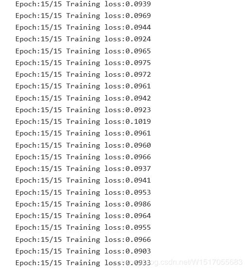
epochs =15  # 迭代次数
batch_size = 128   # 批次大小
sess.run(tf.initialize_all_variables())   # 初始化

for e in range(epochs):
    for idx in range(mnist.train.num_examples // batch_size):
        batch = mnist.train.next_batch(batch_size)  #批次
        imgs = batch[0].reshape((-1,28,28,1)) # reshape

        # 加入噪声
        noisy_images = imgs+noisy_factor*np.random.randn(*imgs.shape)
        noisy_images = np.clip(noisy_images,0.0, 1.0)
        batch_cost, _ = sess.run([cost, optimizer],feed_dict={input_x:noisy_images, target_x:imgs})
        print("Epoch:{}/{}".format(e+1, epochs), "Training loss:{:.4f}".format(batch_cost))

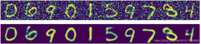
测试模型
首先在测试图片中加入噪声，并输入给自编码器。

fig, axes = plt.subplots(nrows = 2, ncols = 10,figsize = (15, 4)) # matplotlib 画图
imgs = mnist.test.images[10:20] 

noisy_imgs = imgs+noisy_factor*np.random.randn(*imgs.shape)  # 加入噪声点
noisy_imgs = np.clip(noisy_imgs,0.0,1.0)  # 每个像素值在 0.0 - 1.0之间

reconstructed = sess.run(output_y,feed_dict={input_x:noisy_imgs.reshape((10,28,28,1))})

for images, row in zip([noisy_imgs,reconstructed],axes):
    for img, ax in zip(images,row):
        ax.imshow(img.reshape((28,28)))
        ax.get_xaxis().set_visible(False)
        ax.get_yaxis().set_visible(False)
fig.tight_layout(pad=0.1)

参考博客：https://www.cnblogs.com/yxnchinahlj/p/9526476.html