01_行销（Marketing）里的有用的KPI-转换率 （Conversion Rate）

在这篇文章里我会用一个Kaggle的数据集来演示怎么计算行销学里比较有用的KPI计算。数据来源于 bank-additional-full.csv。这里我们着重讲数字行销（digital marketing）里比较重要的几个概念。例如，您可以基于个人归因逻辑，分析通过不同的社交网络服务（例如Facebook，LinkedIn和Instagram）产生的销售额。我们还可以分析通过此类营销渠道获得了多少客户，并查看各个数字营销活动的CPA和产生的价值。

• CTR （Click-through-rate）: 点击率是查看看你的广告然后继续点击广告的用户所占的百分比。它可以衡量在线营销为网站带来流量方面的有效性

• MQL (marketing qualified leads): 营销合格的潜在客户。这些符合市场营销条件的潜在客户（MQL）是可以根据其特征准备出售并符合特定业务标准以成为可能进行购买的客户的潜在客户。当开始营销这些合格的潜在客户时，我们还应该查看转化率。

• Conversion Rate： 转换率可被定义为，采取所需行动的访客百分比，也可以理解为转化率是转化为活跃客户的潜在客户的百分比。当访客进入网站浏览并最终有透过点击行动呼吁(Call to action , CTA)按钮的方式，完成某个目的的比例，大多数人常会误会完成下单购买才可称为转换，但在不同形式的网站中，访客能为网站产生价值的方式不尽相同，转换的型态也不同。
  
  如果我们想查看在网站上注册的潜在客户的百分比，则公式变为
  
  下面是一个怎么用Python计算的例子

# This Python 3 environment comes with many helpful analytics libraries installed
# It is defined by the kaggle/python Docker image: https://github.com/kaggle/docker-python
# For example, here's several helpful packages to load

import numpy as np # linear algebra
import pandas as pd # data processing, CSV file I/O (e.g. pd.read_csv)

# Input data files are available in the read-only "../input/" directory
# For example, running this (by clicking run or pressing Shift+Enter) will list all files under the input directory

import os
for dirname, _, filenames in os.walk('/kaggle/input'):
    for filename in filenames:
        print(os.path.join(dirname, filename))

# You can write up to 5GB to the current directory (/kaggle/working/) that gets preserved as output when you create a version using "Save & Run All" 
# You can also write temporary files to /kaggle/temp/, but they won't be saved outside of the current session

/kaggle/input/bank-marketing/bank-additional-full.csv
/kaggle/input/bank-marketing/bank-additional-names.txt

Load the packages

import matplotlib.pyplot as plt
import pandas as pd
%matplotlib inline

Load the dataset

df = pd.read_csv('../input/bank-marketing/bank-additional-full.csv', sep=';')

df.head(3)

	age	job	marital	education	default	housing	loan	contact	month	day_of_week	...	campaign	pdays	previous	poutcome	emp.var.rate	cons.price.idx	cons.conf.idx	euribor3m	nr.employed	y
0	56	housemaid	married	basic.4y	no	no	no	telephone	may	mon	...	1	999	0	nonexistent	1.1	93.994	-36.4	4.857	5191.0	no
1	57	services	married	high.school	unknown	no	no	telephone	may	mon	...	1	999	0	nonexistent	1.1	93.994	-36.4	4.857	5191.0	no
2	37	services	married	high.school	no	yes	no	telephone	may	mon	...	1	999	0	nonexistent	1.1	93.994	-36.4	4.857	5191.0	no

3 rows ?? 21 columns

Change category variable to numeric 0 and 1

df['conversion'] = df['y'].apply(lambda x: 1 if x == 'yes' else 0)
df.head(3)

	age	job	marital	education	default	housing	loan	contact	month	day_of_week	...	pdays	previous	poutcome	emp.var.rate	cons.price.idx	cons.conf.idx	euribor3m	nr.employed	y	conversion
0	56	housemaid	married	basic.4y	no	no	no	telephone	may	mon	...	999	0	nonexistent	1.1	93.994	-36.4	4.857	5191.0	no	0
1	57	services	married	high.school	unknown	no	no	telephone	may	mon	...	999	0	nonexistent	1.1	93.994	-36.4	4.857	5191.0	no	0
2	37	services	married	high.school	no	yes	no	telephone	may	mon	...	999	0	nonexistent	1.1	93.994	-36.4	4.857	5191.0	no	0

3 rows ?? 22 columns

Aggregate Conversion Rate

print('total conversions: %i out of %i' % (df.conversion.sum(), df.shape[0]))
print('conversion rate: %0.2f%%' % (df.conversion.sum() / df.shape[0] * 100.0))

total conversions: 4640 out of 41188
conversion rate: 11.27%

Conversion Rates by Number of Campaigns

Conversion Numbers

pd.DataFrame(
    df.groupby(
        by='campaign'
    )['conversion'].sum()
).head()

	conversion
campaign
1	2300
2	1211
3	574
4	249
5	120

Numbers of members in different campaigns

pd.DataFrame(
    df.groupby(
        by='campaign'
    )['conversion'].count()
).head()

	conversion
campaign
1	17642
2	10570
3	5341
4	2651
5	1599

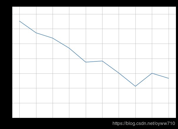
Count conversion rates by campaign

conversions_by_contacts = df.groupby(
    by='campaign'
)['conversion'].sum() / df.groupby(
    by='campaign'
)['conversion'].count() * 100.0

conversions_by_contacts.head()

campaign
1    13.037071
2    11.456954
3    10.747051
4     9.392682
5     7.504690
Name: conversion, dtype: float64

ax = conversions_by_contacts[:10].plot(
    grid=True,
    figsize=(10, 7),
    xticks=conversions_by_contacts.index[:10],
    title='Conversion Rates by Campaign'
)

ax.set_ylim([0, 15])
ax.set_xlabel('number of contacts')
ax.set_ylabel('conversion rate (%)')

plt.show()

Conversion Rates by Age

conversions_by_age = df.groupby(
    by='age'
)['conversion'].sum() / df.groupby(
    by='age'
)['conversion'].count() * 100.0

pd.DataFrame(conversions_by_age).head()

	conversion
age
17	40.000000
18	42.857143
19	47.619048
20	35.384615
21	28.431373

ax = conversions_by_age.plot(
    grid=True,
    figsize=(10, 7),
    title='Conversion Rates by Age'
)

ax.set_xlabel('age')
ax.set_ylabel('conversion rate (%)')

plt.show()

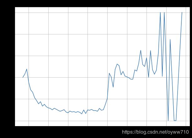
Next we look at age bucket for conversion rates

Create Age Groups

df['age_group'] = df['age'].apply(
    lambda x: '[18, 30)' if x < 30 else '[30, 40)' if x < 40 \
        else '[40, 50)' if x < 50 else '[50, 60)' if x < 60 \
        else '[60, 70)' if x < 70 else '70+'
)

df.head(3)

	age	job	marital	education	default	housing	loan	contact	month	day_of_week	...	previous	poutcome	emp.var.rate	cons.price.idx	cons.conf.idx	euribor3m	nr.employed	y	conversion	age_group
0	56	housemaid	married	basic.4y	no	no	no	telephone	may	mon	...	0	nonexistent	1.1	93.994	-36.4	4.857	5191.0	no	0	[50, 60)
1	57	services	married	high.school	unknown	no	no	telephone	may	mon	...	0	nonexistent	1.1	93.994	-36.4	4.857	5191.0	no	0	[50, 60)
2	37	services	married	high.school	no	yes	no	telephone	may	mon	...	0	nonexistent	1.1	93.994	-36.4	4.857	5191.0	no	0	[30, 40)

3 rows ?? 23 columns

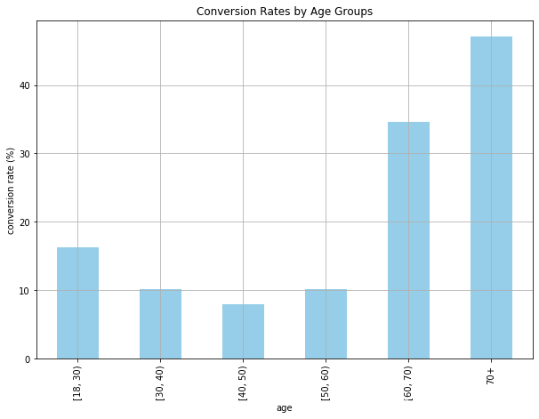
Conversion Rate by Age Group

conversions_by_age_group = df.groupby(
    by='age_group'
)['conversion'].sum() / df.groupby(
    by='age_group'
)['conversion'].count() * 100.0

pd.DataFrame(conversions_by_age_group).head()

	conversion
age_group
70+	47.121535
[18, 30)	16.263891
[30, 40)	10.125162
[40, 50)	7.923238
[50, 60)	10.157389

ax = conversions_by_age_group.loc[
    ['[18, 30)', '[30, 40)', '[40, 50)', '[50, 60)', '[60, 70)', '70+']
].plot(
    kind='bar',
    color='skyblue',
    grid=True,
    figsize=(10, 7),
    title='Conversion Rates by Age Groups'
)

ax.set_xlabel('age')
ax.set_ylabel('conversion rate (%)')

plt.show()

Conversions vs. Non-Conversions On Different Features

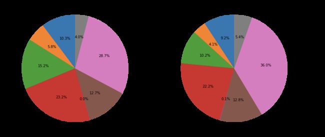
Marital Status

conversions_by_marital_status_df = pd.pivot_table(df, values='y', index='marital', columns='conversion', aggfunc=len)
conversions_by_marital_status_df.columns = ['non_conversions', 'conversions']
conversions_by_marital_status_df

	non_conversions	conversions
marital
divorced	4136	476
married	22396	2532
single	9948	1620
unknown	68	12

conversions_by_marital_status_df.plot(
    kind='pie',
    figsize=(15, 7),
    startangle=90,
    subplots=True,
    autopct=lambda x: '%0.1f%%' % x
)

plt.show()

Education

conversions_by_education_df = pd.pivot_table(df, values='y', index='education', columns='conversion', aggfunc=len)
conversions_by_education_df.columns = ['non_conversions', 'conversions']
conversions_by_education_df

	non_conversions	conversions
education
basic.4y	3748	428
basic.6y	2104	188
basic.9y	5572	473
high.school	8484	1031
illiterate	14	4
professional.course	4648	595
university.degree	10498	1670
unknown	1480	251

conversions_by_education_df.plot(
    kind='pie',
    figsize=(15, 7),
    startangle=90,
    subplots=True,
    autopct=lambda x: '%0.1f%%' % x,
    legend=False
)

plt.show()

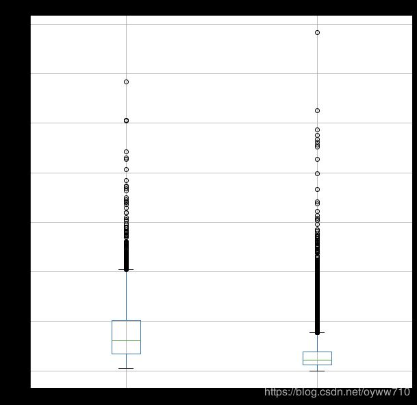
Last Contact Duration

df.groupby('conversion')['duration'].describe()

	count	mean	std	min	25%	50%	75%	max
conversion
0	36548.0	220.844807	207.096293	0.0	95.0	163.5	279.00	4918.0
1	4640.0	553.191164	401.171871	37.0	253.0	449.0	741.25	4199.0

duration_df = pd.concat([
    df.loc[df['conversion'] == 1, 'duration'].reset_index(drop=True), 
    df.loc[df['conversion'] == 0, 'duration'].reset_index(drop=True)
], axis=1)

duration_df.columns = ['conversions', 'non_conversions']

duration_df = duration_df / (60*60)
duration_df

	conversions	non_conversions
0	0.437500	0.072500
1	0.289444	0.041389
2	0.407500	0.062778
3	0.160833	0.041944
4	0.128056	0.085278
...	...	...
36543	NaN	0.070556
36544	NaN	0.031111
36545	NaN	0.106389
36546	NaN	0.052500
36547	NaN	0.066389

36548 rows ?? 2 columns

ax = duration_df.plot(
    kind='box',
    grid=True,
    figsize=(10, 10),
)

ax.set_ylabel('last contact duration (hours)')
ax.set_title('Last Contact Duration')

plt.show()

Conversions by Age Groups & Marital Status

age_marital_df = df.groupby(['age_group', 'marital'])['conversion'].sum().unstack('marital').fillna(0)

age_marital_df.head(3)

marital	divorced	married	single	unknown
age_group
70+	64.0	151.0	6.0	0.0
[18, 30)	12.0	158.0	751.0	1.0
[30, 40)	128.0	897.0	684.0	6.0

age_marital_df = age_marital_df.divide(
    df.groupby(
        by='age_group'
    )['conversion'].count(), 
    axis=0
)

age_marital_df

marital	divorced	married	single	unknown
age_group
70+	0.136461	0.321962	0.012793	0.000000
[18, 30)	0.002117	0.027871	0.132475	0.000176
[30, 40)	0.007557	0.052958	0.040383	0.000354
[40, 50)	0.011970	0.054627	0.012350	0.000285
[50, 60)	0.017342	0.077674	0.006412	0.000146
[60, 70)	0.037293	0.301105	0.006906	0.001381

ax = age_marital_df.loc[
    ['[18, 30)', '[30, 40)', '[40, 50)', '[50, 60)', '[60, 70)', '70+']
].plot(
    kind='bar', 
    grid=True,
    figsize=(10,7)
)

ax.set_title('Conversion rates by Age & Marital Status')
ax.set_xlabel('age group')
ax.set_ylabel('conversion rate (%)')

plt.show()

ax = age_marital_df.loc[
    ['[18, 30)', '[30, 40)', '[40, 50)', '[50, 60)', '[60, 70)', '70+']
].plot(
    kind='bar', 
    stacked=True,
    grid=True,
    figsize=(10,7)
)

ax.set_title('Conversion rates by Age & Marital Status')
ax.set_xlabel('age group')
ax.set_ylabel('conversion rate (%)')

plt.show()