Homography 单应性变换详解

Homography 单应性变换详解

综合了一些资料，整理一下关于Homography的知识，先说结论，Homography就是投影变换，对2D变换有了解的，可以直接跳到最下面看

Homography ：一个例子

样例摘自这里

上图中的红点标明了左右图中对应的点，Homography就是将一幅图中的点映射到另一幅图中它的对应点的映射，可以通过一个3乘3矩阵表示
$$\left[\begin{array}{ccc}{h}_1& h_2& h_3\\ h_4& h_5& h_6\\ h_7& h_8& h_9\end{array}\right]$$
当我们有了这个矩阵，就可以把第一幅图片映射成第二幅图片的视角

右图就是将前面一张图片的左图映射成本图中左图视角的结果

从2D变换说起

了解过2D变换的都知道，2D变换包括2维平面上的平移、旋转、缩放等等，其中旋转和缩放本质上就是线性变换，这一点在线性变换的本质中讲的清清楚楚

旋转

平面坐标系上的一个形状

将其沿坐标轴逆时针旋转30°可得

设旋转前某个点的坐标为$(x,y)$,旋转后其对应点坐标为$(x^{\prime },y^{\prime })$，则有
$$\left[\begin{array}{c}{x}^{\prime }\\ y^{\prime }\end{array}\right]=\left[\begin{array}{cc}\cos 30°& -\sin 30°\\ \sin 30°& \cos 30°\end{array}\right]\left[\begin{array}{c}x\\ y\end{array}\right]$$

缩放

平面坐标系上的一个形状

将其宽放大1.5倍，高放大2倍

设变换前某个点的坐标为$(x,y)$,旋转后其对应点坐标为$(x^{\prime },y^{\prime })$，则有
$$\left[\begin{array}{c}{x}^{\prime }\\ y^{\prime }\end{array}\right]=\left[\begin{array}{cc}1.5& 0\\ 0& 2\end{array}\right]\left[\begin{array}{c}x\\ y\end{array}\right]$$

线性变换与矩阵

矩阵和线性变换是一一对应的，任意的线性变换总能找到一个矩阵，任意的矩阵也代表一个线性变换，而矩阵之间的乘法即是线性变换的复合，比如记上述的旋转变换的矩阵为$W_1$，缩放变换的矩阵为$W_2$，那么$W_1{W}_2$就是先缩放后旋转，$W_2{W}_1$就是先旋转后缩放，这是因为右边的矩阵总是先作用到向量上的，此外还有一些基本认识

• 正交矩阵都代表了旋转
• 变换矩阵的每一列分别是原先的基变换后的向量

平移

线性变换保持原点不变的特点使得平移无法被表示出来，但是通过特殊的方法我们也可以使用线性变换来表达平移，即更换2D点的表示方式

在我的这篇博客中，记录了2D点的表示方式，包括

• 二元组表示，$\mathbf{x}=(x,y)\in R$
• 齐次坐标表示，$\mathbf{x}=(x,y,w)$
• 非齐次坐标表示，$\bar{\mathbf{x}}=(x,y,1)$，$\mathbf{x}=w\bar{\mathbf{x}}$，可以与直线的其次坐标表示点乘获得直线方程

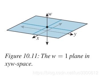
当我们使用非齐次坐标表示的时候，平移也可以通过线性变换来表达，此时我们可以将平面看作$xyw$空间中由$w=1$定义的一个子集

此时可验证
$$\left[\begin{array}{c}x+c\\ y+f\\ 1\end{array}\right]=\left[\begin{array}{ccc}1& 0& c\\ 0& 1& f\\ 0& 0& 1\end{array}\right]\left[\begin{array}{c}x\\ y\\ 1\end{array}\right]$$
这就通过线性变换来表达了平移，像这样限制在平面$w=1$内的变换，称为平面的仿射变换，实际上就是线性变换+平移变换

而且旋转和缩放也很容易拓展到这种形式
$$\left[\begin{array}{c}{x}^{\prime }\\ y^{\prime }\\ 1\end{array}\right]=\left[\begin{array}{ccc}\cos 30°& -\sin 30°& 0\\ \sin 30°& \cos 30°& 0\\ 0& 0& 1\end{array}\right]\left[\begin{array}{c}x\\ y\\ 1\end{array}\right]$$

$$\left[\begin{array}{c}{x}^{\prime }\\ y^{\prime }\\ 1\end{array}\right]=\left[\begin{array}{ccc}1.5& 0& 0\\ 0& 2& 0\\ 0& 0& 1\end{array}\right]\left[\begin{array}{c}x\\ y\\ 1\end{array}\right]$$

且此时，线性变换依然由矩阵决定，旋转、平移、缩放等变换的复合可以通过求它们对应矩阵的乘积得到

窗口变换

窗口变换将一个轴向对其的矩形移动到另一个位置

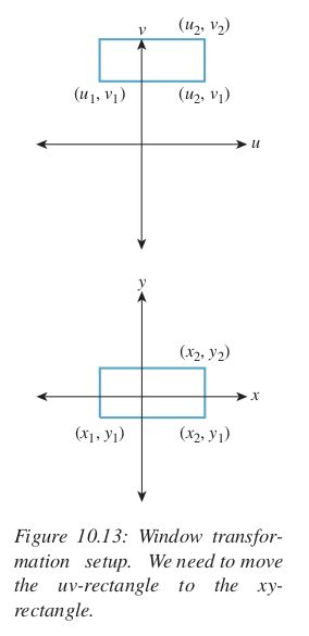
有了三个点的对应关系之后，我们就可以通过以下方法来确定这个变换

注意到我们这里是在三维空间上确定一个线性变换，所以需要三个线性无关向量的对应，而不是之前说的两个

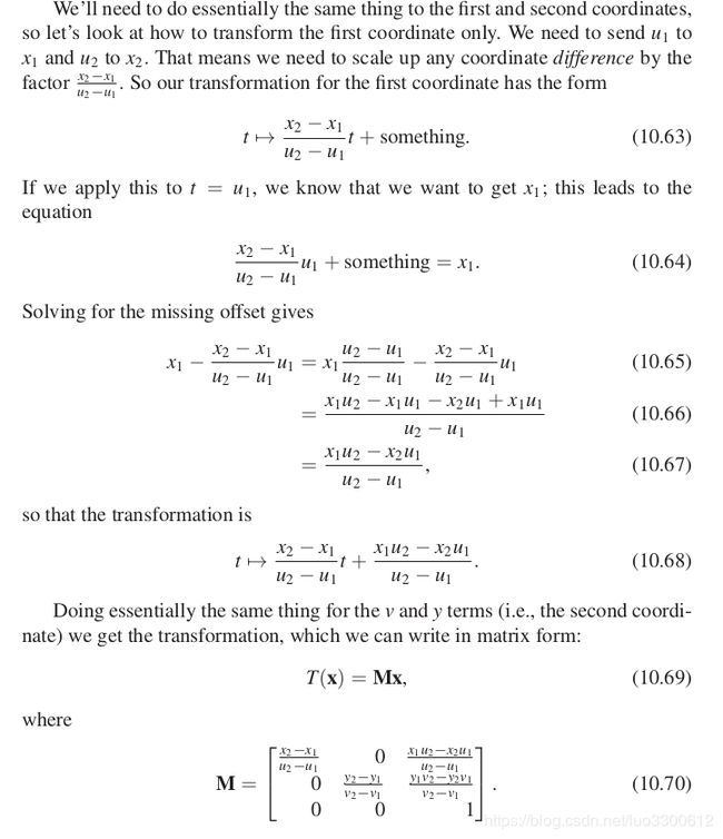
确定一个2D变换

如果我们只知道一个变换将图形逆时针旋转$\theta$，那我们如何确定这个变换呢？
对于这种情况，根据正交变换的固定形式可以直接确定为
$$\left[\begin{array}{cc}\cos \theta & -\sin \theta \\ \sin \theta & \cos \theta \end{array}\right]$$
将宽扩大2倍，高扩大3倍，则是
$$\left[\begin{array}{cc}3& 0\\ 0& 2\end{array}\right]$$
事实上，变换的矩阵每列分别是$(1,0)$和$(0,1)$经过变换之后的坐标，比如旋转中$(1,0)$变成了$(\cos \theta ,-\sin \theta )$，$(0,1)$变成了$(-\sin \theta ,\cos \theta )$，因此变换的矩阵就由这两个向量按列组成，容易验证缩放的例子也是一样的。且当给出两个线性无关的向量$(x_1,y_1),(x_2,y_2)$以及它们变换后的位置$(u_1,v_1),(u_2,v_2)$之后就可以确定一个2维的线性变换

容易验证单位矩阵作的是恒等变换
$$\left[\begin{array}{c}x\\ y\end{array}\right]=\left[\begin{array}{cc}1& 0\\ 0& 1\end{array}\right]\left[\begin{array}{c}x\\ y\end{array}\right]$$
因此如果我们先作了一个线性变换$A$，为了还原这个变换，只要求其逆矩阵即可$x=A^{-1}Ax$，$A^{-1}$也就是它的逆变换
于是，对于一个general的问题：为了将$(x_1,y_1),(x_2,y_2)$变换为$(u_1,v_1),(u_2,v_2)$，变换的矩阵形式是怎样的？只需要先将$(x_1,y_1),(x_2,y_2)$变换为$(1,0),(0,1)$，易知这个变换的矩阵为
$${\left[\begin{array}{cc}{x}_1& x_2\\ y_1& y_2\end{array}\right]}^{-1}$$
也就是将$(1,0),(0,1)$变换为$(x_1,y_1),(x_2,y_2)$的逆变换

再将$(1,0),(0,1)$变换为$(u_1,v_1),(u_2,v_2)$，即
$$\left[\begin{array}{cc}{u}_1& u_2\\ v_1& v_2\end{array}\right]$$
然后将两者复合即可得到所求变换$W$为
$$W=\left[\begin{array}{cc}{u}_1& u_2\\ v_1& v_2\end{array}\right]{\left[\begin{array}{cc}{x}_1& x_2\\ y_1& y_2\end{array}\right]}^{-1}$$

二维的例子作为引子，为的是引出当我们使用非齐次坐标的时候，可以使用同样的方法来确定一个变换

确定一个3D变换

平移虽然是在2维平面上的一个变换，但实际上是一个三维线性变换，仿照确定2D线性变换的方法，我们可以确定一个3D线性变换，如之前的窗口变换所示，为了将$(u_1,v_1),(u_2,v_2),(u_2,v_1)$变换到$(x_1,y_1),(x_2,y_2),(x_2,y_1)$，先将$(u_1,v_1),(u_2,v_2),(u_2,v_1)$变换到$(1,0,0),(0,1,0),(0,0,1)$
$${\left[\begin{array}{ccc}{u}_1& u_2& u_2\\ v_1& v_2& v_1\\ 1& 1& 1\end{array}\right]}^{-1}$$
然后将$(1,0,0),(0,1,0),(0,0,1)$变换到$(x_1,y_1),(x_2,y_2),(x_2,y_1)$
$$\left[\begin{array}{ccc}{x}_1& x_2& x_2\\ y_1& y_2& y_1\\ 1& 1& 1\end{array}\right]$$
然后将两者复合即可得到所求变换$W$为
$$\left[\begin{array}{ccc}{x}_1& x_2& x_2\\ y_1& y_2& y_1\\ 1& 1& 1\end{array}\right]{\left[\begin{array}{ccc}{u}_1& u_2& u_2\\ v_1& v_2& v_1\\ 1& 1& 1\end{array}\right]}^{-1}$$

利用这个方法，我们可以更简单地确定一个变换，比如，我们要确定一个绕(2,4)逆时针旋转30°的变换，我们可能想先将(2,4)平移到原点，然后旋转，然后再把原点平移回(2,4)，而实际上我们在平面上取三个点使得它们的非齐次表示线性无关，然后计算出它们平移之后的位置就可以通过上面的方法来求得变换了

再谈确定变换

之前我们发现缩放和旋转可以由两个线性无关的向量确定，平移和窗口变换（实际上就是平移+线性变换的一种特殊形式）可以由三个非齐次表示线性无关的向量确定，我们把所有结论总结在下面

• 2D空间中的线性变换可以由两个线性无关的向量确定
• 仿射变换可以由非共线的任意三个点（实际上就是非齐次坐标线性无关）决定
• 平面透视变换（将在之后介绍）由四个（其中任意三个点均不共线）确定

OpenCV中的仿射变换

之前所讨论的变换写成三维矩阵乘法的时候，我们能发现所有的矩阵最后一行均是$[0,0,1]$，而且之前讨论的变换均属于仿射变换，由于仿射变换的最后一行均是$[0,0,1]$，所以我们储存一个仿射变换的时候只要存储其前两行就行了，opencv应用一个仿射变换，就是传入一个2*3的矩阵


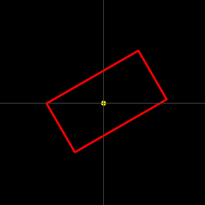
回到开头的例子，当我想要绕原点旋转矩形的时候

我只需要计算出能表达它的仿射矩阵即可，因为opencv以左上角为原点，所以我先将图片中心平移到原点
$$\left[\begin{array}{ccc}1& 0& -150\\ 0& 1& -150\\ 0& 0& 1\end{array}\right]$$
然后旋转
$$\left[\begin{array}{ccc}\cos 30°& \sin 30°& 0\\ -\sin 30°& \cos 30°& 0\\ 0& 0& 1\end{array}\right]$$
值得注意的是，你对比可以发现，这里的旋转矩阵与之前的有点不一样，这是因为opencv的y轴正方向是向下的，与我们平常使用y轴向上是不一样的
最后将原点平移回去
$$\left[\begin{array}{ccc}1& 0& 150\\ 0& 1& 150\\ 0& 0& 1\end{array}\right]$$
因为可以用计算机直接算矩阵乘法，所以我选择了这种求变换的方法，代码如下

import cv2
import numpy as np

img = np.zeros((300, 300, 3), dtype=np.uint8)
origin = (150, 150)

cv2.rectangle(img, (80, 110), (220, 190), [0, 0, 255], 2)  # 画矩形
cv2.circle(img, origin, 2, [0, 255, 255], 2)  # 标原点

theta = 30 / 180 * np.pi
W1 = np.array([[1, 0, -150], [0, 1, -150], [0, 0, 1]])
W2 = np.array([[np.cos(theta), np.sin(theta), 0], [-np.sin(theta), np.cos(theta), 0], [0, 0, 1]])
W3 = np.array([[1, 0, 150], [0, 1, 150], [0, 0, 1]])
W = W3.dot(W2.dot(W1))

img = cv2.warpAffine(img, W[:2, :], img.shape[:2])

# 画坐标轴
cv2.line(img, (0, 150), (300, 150), [70, 70, 70], 1)
cv2.line(img, (150, 0), (150, 300), [70, 70, 70], 1)
cv2.imshow("Window1", img)
cv2.waitKey(0)

结果就和开始的一样

当然，也不必这么麻烦，opencv里给出了直接取得绕某点旋转的仿射变换矩阵的方法

W = cv2.getRotationMatrix2D(origin, 30,1)

可以直接得到一个2*3的矩阵，所以上面的写法等价于

import cv2
import numpy as np

img = np.zeros((300, 300, 3), dtype=np.uint8)
origin = (150, 150)

cv2.rectangle(img, (80, 110), (220, 190), [0, 0, 255], 2)  # 画矩形
cv2.circle(img, origin, 2, [0, 255, 255], 2)  # 标原点

W = cv2.getRotationMatrix2D(origin, 30,1)

img = cv2.warpAffine(img, W[:2, :], img.shape[:2])

# 画坐标轴
cv2.line(img, (0, 150), (300, 150), [70, 70, 70], 1)
cv2.line(img, (150, 0), (150, 300), [70, 70, 70], 1)
cv2.imshow("Window1", img)
cv2.waitKey(0)

更一般的变换

问题来了，如果变换矩阵的最后一行不是$[0,0,1]$会发生什么？

首先看看是$[0,0,1]$会发生什么

对于任意一个$w=1$上的点$(x,y,1)$，任何仿射变换
$$\left[\begin{array}{ccc}a& b& c\\ d& e& f\\ 0& 0& 1\end{array}\right]\left[\begin{array}{c}x\\ y\\ 1\end{array}\right]=\left[\begin{array}{c}ax+by+c\\ dx+ey+f\\ 1\end{array}\right]$$
变换后的点仍然在$w=1$上

如果最后一行不是$[0,0,1]$，可能将点变换到$w=1$之外，但我们可以通过齐次变换将其变换到$w=1$上

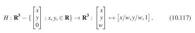
几何上看，就是连接原点和目标点，将目标点变换为直线与$w=1$的交点，注意，这样对$w=0$的点不适用

上述的两个变换（矩阵最后一行不是$[0,0,1]$外加一个齐次变换）的复合称为投影变换（projection transformation），它就是本文要解释的核心概念单应性变换（Homography）的同义词¹，它包含了之前所提到的所有变换，这是《计算机图形学原理及实践第三版》的定义，可能它特别强调最后结果在$w=1$上的这个特点，在找到的其他材料中¹²³，对Homography的定义如开头所述就是一个任意的三维矩阵，并不包括后来的齐次变换，本文也采样这种定义
$$H=\left[\begin{array}{ccc}{h}_1& h_2& h_3\\ h_4& h_5& h_6\\ h_7& h_8& h_9\end{array}\right]$$

但实际上，8个参数即可确定一个Homography，因为当$H_1=c{H}_2$（c是非0常数）时，它们是一样的Homography，这很容易证明，如果
$$\left[\begin{array}{ccc}{h}_1& h_2& h_3\\ h_4& h_5& h_6\\ h_7& h_8& h_9\end{array}\right]\left[\begin{array}{c}x\\ y\\ 1\end{array}\right]=\left[\begin{array}{c}u\\ v\\ w\end{array}\right]$$
那么
$$\left[\begin{array}{ccc}c{h}_1& c{h}_2& c{h}_3\\ c{h}_4& c{h}_5& c{h}_6\\ c{h}_7& c{h}_8& c{h}_9\end{array}\right]\left[\begin{array}{c}x\\ y\\ 1\end{array}\right]=\left[\begin{array}{c}cu\\ cv\\ cw\end{array}\right]$$
经过齐次变换之后，结果一样，都是$[u/w,v/w,1]$，因此OpenCV里将Homography矩阵的右下角记为1⁴

>>>import cv2
>>>import numpy as np
>>>pts_src = np.array([[141, 131], [480, 159], [493, 630], [64, 601]])
>>>pts_dst = np.array([[318, 256], [534, 372], [316, 670], [73, 473]])
>>>h, status = cv2.findHomography(pts_src, pts_dst) # 根据四个点间的关系找到Homography映射
>>>print(h)
[[ 4.34043935e-01 -4.19622184e-01  2.91709494e+02]
 [ 1.46491654e-01  4.41418278e-01  1.61369294e+02]
 [-3.62463336e-04 -9.14274844e-05  1.00000000e+00]]

确定homography和输出的尺寸，就可以这样对图片应用homography

im_dst = cv2.warpPerspective(im_src, h, size)

此外，Homography可以分解为两个变换的乘积⁵
$$\left[\begin{array}{ccc}{h}_1& h_2& h_3\\ h_4& h_5& h_6\\ h_7& h_8& 1\end{array}\right]=\left[\begin{array}{ccc}{h}_1-h_3{h}_7& h_2-h_3{h}_8& h_3\\ h_4-h_6{h}_7& h_5-h_6{h}_8& h_6\\ 0& 0& 1\end{array}\right]\left[\begin{array}{ccc}1& 0& 0\\ 0& 1& 0\\ h_7& h_8& 1\end{array}\right]$$
左边显然是一个仿射变换，问题是右边是什么呢？
尝试将右边作用在某点上
$$\left[\begin{array}{ccc}1& 0& 0\\ 0& 1& 0\\ h_7& h_8& 1\end{array}\right]\left[\begin{array}{c}x\\ y\\ 1\end{array}\right]=\left[\begin{array}{c}x\\ y\\ h_{7}x+h_{8}y+1\end{array}\right]$$
因为我们最后还是研究在$w=1$上的点，所以对其进行齐次变换得到$(x/k,y/k,1),k=h_{7}x+h_{8}y+1$，它将直线$h_{7}x+h_{8}y+1=0$变换到了无穷远处，其余的特点在第五处引用中进一步了解

另外OpenCV中还有一个变换叫Perspective transformation（透视变换），其实就是Homography

结论

• Homography=projection transformation=perspective transformation

---

1. https://ags.cs.uni-kl.de/fileadmin/inf_ags/3dcv-ws11-12/3DCV_WS11-12_lec04.pdf ↩︎ ↩︎

2. https://math.stackexchange.com/questions/1319680/affine-vs-projective-tranformation ↩︎

3. https://www.learnopencv.com/homography-examples-using-opencv-python-c/ ↩︎

4. 3 ↩︎

5. https://math.stackexchange.com/questions/1319680/affine-vs-projective-tranformation
   https://en.wikipedia.org/wiki/Homography ↩︎