SCENIC—Single Cell rEgulatory Network Inference and Clustering

SCENIC是一种基于单细胞RNA-seq数据推断基因调控网络及其相关细胞状态的工具

这里介绍的步骤方法是针对在R环境中（GENIE3），主要是GENIE3/GRNBoost这两种方法的选择，数据量大的推荐使用GRNBoost（in Python），参考https://www.jianshu.com/p/eccfe2d1b2c7

SCENIC分析步骤：

建立基因调控网络

1. 根据每个转录因子的共表达确定它的潜在靶点；
   ·对表达矩阵进行过滤+running GENIE3/GRNBoost
   ·将上一步骤中得到的targets构建共表达模型
2. 根据DNA motif分析，挑选潜在的直接结合的靶点（regulons: transcription factors (TFs) and their target genes, together defining a regulon）；

鉴定细胞状态及其调控元件

1. 对每一个细胞分析网络活性；
   ·对细胞中的regulons进行打分
   ·可选步骤：将network activity转换成ON/OFF格式
2. 根据基因调控网络活性鉴定稳定细胞状态+对结果进行进一步探索；

1. 输入文件格式：single-cell RNA-seq expression matrix

a) .loom文件

#.loom文件能够直接导入SCENIC
# 下载.loom文件: download.file("http://loom.linnarssonlab.org/clone/Previously%20Published/Cortex.loom", "Cortex.loom") 
loomPath <- "Cortex.loom"

#导入数据
library(SCopeLoomR) 
loom <- open_loom(loomPath, mode="r") 
exprMat <- get_dgem(loom) 
cellInfo <- get_cellAnnotation(loom) 
close_loom(loom)

b) 10X/CellRanger下机数据
load the CellRanger output into R

c) 其他R对象（e.g. Seurat、SingleCellExperiment）

#for a SingleCellExperiment object
sce <- load_as_sce(loomPath) # any SingleCellExperiment object exprMat <- counts(sce) 
cellInfo <- colData(sce)

#for a Seurat object
# 首先选择你要提取的细胞 
cells.use <- WhichCells(object = immune.combined, ident = 3) 
# 这里的assay指的是你要提取的表达矩阵类型 
expr <- GetAssayData(object = immune.combined, assay= "RNA", slot = "data")[, cells.use] 
# 转换格式 
expr <- as(Class = 'matrix', object = expr)
cellInfo <- data.frame(seuratCluster=Idents(seuratObject))

d) GEO数据

# dir.create("SCENIC_MouseBrain"); setwd("SCENIC_MouseBrain") # if needed # (This may take a few minutes) 
if (!requireNamespace("GEOquery", quietly = TRUE)) BiocManager::install("GEOquery") 

library(GEOquery) 
geoFile <- getGEOSuppFiles("GSE60361", makeDirectory=FALSE) gzFile <- grep("Expression", basename(rownames(geoFile)), value=TRUE) 
txtFile <- gsub(".gz", "", gzFile) 
gunzip(gzFile, destname=txtFile, remove=TRUE)

library(data.table) 
geoData <- fread(txtFile, sep="\t") 
geneNames <- unname(unlist(geoData[,1, with=FALSE])) 
exprMatrix <- as.matrix(geoData[,-1, with=FALSE]) 
rm(geoData) 
dim(exprMatrix) 
rownames(exprMatrix) <- geneNames 
exprMatrix <- exprMatrix[unique(rownames(exprMatrix)),] exprMatrix[1:5,1:4] 

# Remove file downloaded: 
file.remove(txtFile)

cellLabels <- paste(file.path(system.file('examples', package='AUCell')), "mouseBrain_cellLabels.tsv", sep="/") 
cellLabels <- read.table(cellLabels, row.names=1, header=TRUE, sep="\t") 
cellInfo <- as.data.frame(cellLabels) 
colnames(cellInfo) <- "Class"

2. 初始化数据

2.1 数据导入

#创建空文件夹
dir.create("SCENIC_MouseBrain")
setwd("SCENIC_MouseBrain")

#导入数据，这里用到的是包自带数据
loomPath <- system.file(package="SCENIC", "examples/mouseBrain_toy.loom")

library(SCopeLoomR)
loom <- open_loom(loomPath, mode="r")
exprMat <- get_dgem(loom)
cellInfo <- get_cellAnnotation(loom)
close_loom(loom)

dim(exprMat)
## [1] 862 200

2.2 细胞聚类信息/表型数据

#对感兴趣的变量赋予特定的颜色
head(cellInfo)

##                           Class nGene nUMI
## 1772066100_D04     interneurons   170  509
## 1772063062_G01 oligodendrocytes   152  443
## 1772060224_F07        microglia   218  737
## 1772071035_G09    pyramidal CA1   265 1068
## 1772067066_E12 oligodendrocytes    81  273
## 1772066100_B01    pyramidal CA1   108  191

cellInfo <- data.frame(cellInfo)
cellTypeColumn <- "Class"
colnames(cellInfo)[which(colnames(cellInfo)==cellTypeColumn)] <- "CellType"

head(cellInfo)
##                           CellType nGene nUMI
## 1772066100_D04     interneurons   170  509
## 1772063062_G01 oligodendrocytes   152  443
## 1772060224_F07        microglia   218  737
## 1772071035_G09    pyramidal CA1   265 1068
## 1772067066_E12 oligodendrocytes    81  273
## 1772066100_B01    pyramidal CA1   108  191

#创建文件夹int
dir.create("int")
saveRDS(cellInfo, file="int/cellInfo.Rds")

#针对特定变量指定特定颜色
colVars <- list(CellType=c("microglia"="forestgreen", 
                           "endothelial-mural"="darkorange", 
                           "astrocytes_ependymal"="magenta4", 
                           "oligodendrocytes"="hotpink", 
                           "interneurons"="red3", 
                           "pyramidal CA1"="skyblue", 
                           "pyramidal SS"="darkblue"))
colVars$CellType <- colVars$CellType[intersect(names(colVars$CellType), cellInfo$CellType)]
saveRDS(colVars, file="int/colVars.Rds")

#看一下变量的颜色，这里是分成了5个细胞群，每个群用不同的颜色表示
plot.new(); legend(0,1, fill=colVars$CellType, legend=names(colVars$CellType))

2.3 初始化SCENIC设置

library(SCENIC)
org="mgi" # or hgnc, or dmel
dbDir="cisTarget_databases" # RcisTarget databases location
myDatasetTitle="SCENIC example on Mouse brain" # choose a name for your analysis
data(defaultDbNames)
dbs <- defaultDbNames[[org]]
scenicOptions <- initializeScenic(org=org, dbDir=dbDir, dbs=dbs, datasetTitle=myDatasetTitle, nCores=10) 

## Motif databases selected: 
##   mm9-500bp-upstream-7species.mc9nr.feather 
##   mm9-tss-centered-10kb-7species.mc9nr.feather

scenicOptions@inputDatasetInfo$cellInfo <- "int/cellInfo.Rds"
scenicOptions@inputDatasetInfo$colVars <- "int/colVars.Rds"

saveRDS(scenicOptions, file="int/scenicOptions.Rds")

3. 构建基因共表达网络

这一步的目的是基于表达数据推断潜在的转录因子靶点。输入文件是过滤后的表达矩阵，一系列转录因子；输出是相关性矩阵，用于后续构建共表达模型（runSCENIC_1_coexNetwork2modules()）。
这里有两种方法供选择：GENIE3（在R当中进行操作，能够鉴定非线性关系，耗时，计算量很大）和GRNboost（和前面一种方法类似，但耗时少，适合大数据）

3.1 过滤表达矩阵

#Filter by the total number of reads per gene
#Filter by the number of cells in which the gene is detected
#only the genes that are available in RcisTarget databases will be kept

genesKept <- geneFiltering(exprMat, scenicOptions=scenicOptions,
                           minCountsPerGene=3*.01*ncol(exprMat),
                           minSamples=ncol(exprMat)*.01)
                           
exprMat_filtered <- exprMat[genesKept, ]
## [1] 770 200

#删除不需要的
rm(exprMat)

3.2 相关性
GENIE3/GRNboost能够检测到正相关和负相关的基因，为了将这两种相关性区分开，进行这一步处理。

#This step can be run either before/after or simultaneously to GENIE3/GRNBoost
runCorrelation(exprMat_filtered, scenicOptions)

3.3 GENIE3
To run GRNBoost (in Python) instead of GENIE3. See ?exportsForGRNBoost for details
这一步需要时间很长，可以另外开一个窗口单独运行这一步

# Optional: add log (if it is not logged/normalized already)
exprMat_filtered <- log2(exprMat_filtered+1) 

# Run GENIE3
runGenie3(exprMat_filtered, scenicOptions)

4 构建并计算基因调控网络

library(SCENIC)
scenicOptions <- readRDS("int/scenicOptions.Rds")
scenicOptions@settings$verbose <- TRUE
scenicOptions@settings$nCores <- 10
scenicOptions@settings$seed <- 123

#这里为了计算方便，就选择了一个库
scenicOptions@settings$dbs <- scenicOptions@settings$dbs["10kb"] # For toy run

runSCENIC_1_coexNetwork2modules(scenicOptions)
runSCENIC_2_createRegulons(scenicOptions, coexMethod=c("top5perTarget")) #** Only for toy run!!
runSCENIC_3_scoreCells(scenicOptions, exprMat_filtered)

5 可选步骤：

5.1 将network activity转换成ON/OFF格式

#这一步是将前面得到的结果（AUC threshold）在shiny中进行可视化，你可以在其中手动调整阈值
aucellApp <- plotTsne_AUCellApp(scenicOptions, logMat)
savedSelections <- shiny::runApp(aucellApp)

# 感觉就是要更好的将细胞区分开，Save the modified thresholds:
newThresholds <- savedSelections$thresholds
scenicOptions@fileNames$int["aucell_thresholds",1] <- "int/newThresholds.Rds"
saveRDS(newThresholds, file=getIntName(scenicOptions, "aucell_thresholds"))
saveRDS(scenicOptions, file="int/scenicOptions.Rds") 

#调整好新的阈值后，运行
runSCENIC_4_aucell_binarize(scenicOptions)

5.2 根据regulon activity 聚类降维

#这一步关键的参数“number of PCs” and “perplexity” (expected running time: few minutes to hours, depending on the number of cells)
nPcs <- c(5)
scenicOptions@settings$seed <- 123 # same seed for all of them
# Run t-SNE with different settings:
fileNames <- tsneAUC(scenicOptions, aucType="AUC", nPcs=nPcs, perpl=c(5,15,50))
fileNames <- tsneAUC(scenicOptions, aucType="AUC", nPcs=nPcs, perpl=c(5,15,50), onlyHighConf=TRUE, filePrefix="int/tSNE_oHC")
# Plot as pdf (individual files in int/):
fileNames <- paste0("int/",grep(".Rds", grep("tSNE_", list.files("int"), value=T), value=T))

# Using only "high-confidence" regulons (normally similar)
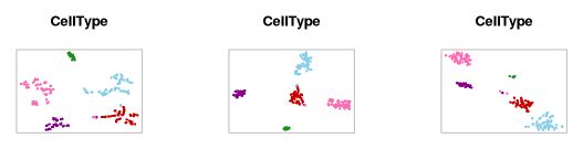
par(mfrow=c(3,3))
fileNames <- paste0("int/",grep(".Rds", grep("tSNE_oHC_AUC", list.files("int"), value=T, perl = T), value=T))
plotTsne_compareSettings(fileNames, scenicOptions, showLegend=FALSE, varName="CellType", cex=.5)

#下面会出图，根据细胞聚类结果选择好的参数值
scenicOptions@settings$defaultTsne$aucType <- "AUC"
scenicOptions@settings$defaultTsne$dims <- 5
scenicOptions@settings$defaultTsne$perpl <- 15
saveRDS(scenicOptions, file="int/scenicOptions.Rds")

6 对产生的中间结果进行进一步探索

6.1 Projection the AUC and TF expression onto t-SNEs

# 首先产生AUCell的交互式界面
#？可能也是对阈值进行调整
logMat <- exprMat # Better if it is logged/normalized
aucellApp <- plotTsne_AUCellApp(scenicOptions, logMat) # default t-SNE
savedSelections <- shiny::runApp(aucellApp)

#这里找到保存的rds对象的路径
print(tsneFileName(scenicOptions))
## [1] "int/tSNE_AUC_05pcs_15perpl.Rds"

tSNE_scenic <- readRDS(tsneFileName(scenicOptions))
aucell_regulonAUC <- loadInt(scenicOptions, "aucell_regulonAUC")

# Show TF expression:
par(mfrow=c(2,3))
AUCell::AUCell_plotTSNE(tSNE_scenic$Y, exprMat, aucell_regulonAUC[onlyNonDuplicatedExtended(rownames(aucell_regulonAUC))[c("Dlx5", "Sox10", "Sox9","Irf1", "Stat6")],], plots="Expression")

6.2 Density plot to detect most likely stable states (higher-density areas in the t-SNE)

library(KernSmooth)
library(RColorBrewer)
dens2d <- bkde2D(tSNE_scenic$Y, 1)$fhat
image(dens2d, col=brewer.pal(9, "YlOrBr"), axes=FALSE)
contour(dens2d, add=TRUE, nlevels=5, drawlabels=FALSE)

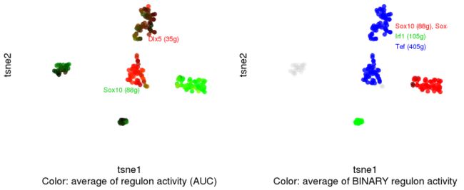
6.3 Show several regulons simultaneously

par(mfrow=c(1,2))

regulonNames <- c( "Dlx5","Sox10")
cellCol <- plotTsne_rgb(scenicOptions, regulonNames, aucType="AUC", aucMaxContrast=0.6)
text(0, 10, attr(cellCol,"red"), col="red", cex=.7, pos=4)
text(-20,-10, attr(cellCol,"green"), col="green3", cex=.7, pos=4)

regulonNames <- list(red=c("Sox10", "Sox8"),
                     green=c("Irf1"),
                     blue=c( "Tef"))
cellCol <- plotTsne_rgb(scenicOptions, regulonNames, aucType="Binary")
text(5, 15, attr(cellCol,"red"), col="red", cex=.7, pos=4)
text(5, 15-4, attr(cellCol,"green"), col="green3", cex=.7, pos=4)
text(5, 15-8, attr(cellCol,"blue"), col="blue", cex=.7, pos=4)

6.4 GRN: Regulon targets and motifs

#查看包含在regulon中的基因
regulons <- loadInt(scenicOptions, "regulons")
regulons[c("Dlx5", "Irf1")]

## $Dlx5
##  [1] "2610203C20Rik" "Adamts17"      "AI854703"      "Arhgef10l"     "Bahcc1"        "Cirbp"         "Cplx1"         "Dlx1"          "Gad1"          "Gadd45gip1"    "Hexim2"        "Igf1"         
## [13] "Iglon5"        "Ltbp3"         "Myt1"          "Npas1"         "Nxph1"         "Peli2"         "Plekha6"       "Prkab1"        "Ptchd2"        "Racgap1"       "Rgs8"          "Robo1"        
## [25] "Rpl34"         "Sema3c"        "Shisa9"        "Slc12a5"       "Slc39a6"       "Spns2"         "Stox2"         "Syt6"          "Unc5d"         "Wnt5a"        
## 
## $Irf1
##   [1] "4930523C07Rik" "Acsl5"         "Adrb1"         "Ahdc1"         "Ahnak"         "Akap1"         "Anxa2"         "Arhgap31"      "Arhgef10l"     "Arhgef19"      "Atg14"         "B2m"          
##  [13] "Bank1"         "Bcl2a1b"       "Cald1"         "Capsl"         "Ccl2"          "Ccl3"          "Ccl7"          "Ccnd1"        "Ccnd3"         "Cd163"         "Cd48"          "Cited2"       
##  [25] "Cmtm6"         "Ctgf"          "Ctnnd1"        "Ctss"          "Ddr2"          "E130114P18Rik" "Egfr"          "Ehd1"          "Esam"          "Fcer1g"        "Fcgr1"         "Fgf14"        
##  [37] "Fstl4"         "Fyb"           "Gabrb1"        "Gadd45g"       "Gja1"          "Gpr34"         "Gramd3"        "H2-K1"         "Hfe"           "Il6ra"         "Irf1"          "Itgb5"        
##  [49] "Kcne4"         "Kcnj16"        "Kcnj2"         "Laptm5"        "Lhfp"          "Map3k5"        "Mdk"           "Med13"         "Midn"          "Mr1"           "Ms4a7"         "Msr1"         
##  [61] "Myh9"          "Nin"           "Nptx1"         "Osbpl6"        "P2ry13"        "Parp12"        "Peli2"         "Plcl2"         "Plekha6"       "Prkab1"        "Rab3il1"       "Rgs5"         
##  [73] "Rhobtb2"       "Rnase4"        "Sepp1"         "Sertad2"       "Sgk3"          "Slamf9"        "Slc4a4"        "Slc7a7"        "Slco5a1"       "Slitrk2"       "Soat1"         "Srgn"         
##  [85] "St3gal6"       "St5"           "St8sia4"       "Stard8"        "Stat6"         "Stk17b"        "Tapbp"         "Tbxas1"        "Tgfa"          "Tgfb3"         "Tmem100"       "Tnfaip3"      
##  [97] "Tnfaip8"       "Trib1"         "Trpm7"         "Txnip"         "Usp2"          "Vgll4"         "Vps37b"        "Zfp36l2"       "Zfp703"

#注意，只有超过十个基因的regulons才会被AUCell计算
regulons <- loadInt(scenicOptions, "aucell_regulons")
head(cbind(onlyNonDuplicatedExtended(names(regulons))))

##       [,1]         
## Tef   "Tef (405g)" 
## Dlx5  "Dlx5 (35g)" 
## Sox9  "Sox9 (150g)"
## Sox8  "Sox8 (97g)" 
## Sox10 "Sox10 (88g)"
## Irf1  "Irf1 (105g)"

#查看TF与靶点之间的联系
regulonTargetsInfo <- loadInt(scenicOptions, "regulonTargetsInfo")
tableSubset <- regulonTargetsInfo[TF=="Stat6" & highConfAnnot==TRUE]
viewMotifs(tableSubset) 

6.5 Regulators for clusters or known cell types

#Average Regulon Activity by cluster
#聚类这里的cluster参数选择可以是CellType，也可以是Seurat对象里面的特定分组
#这里除了可以选择aucell_regulonAUC，还可以选择aucell_binary_nonDupl
regulonAUC <- loadInt(scenicOptions, "aucell_regulonAUC")
regulonAUC <- regulonAUC[onlyNonDuplicatedExtended(rownames(regulonAUC)),]
regulonActivity_byCellType <- sapply(split(rownames(cellInfo), cellInfo$CellType),
                                     function(cells) rowMeans(getAUC(regulonAUC)[,cells]))

regulonActivity_byCellType_Scaled <- t(scale(t(regulonActivity_byCellType), center = T, scale=T))

pheatmap::pheatmap(regulonActivity_byCellType_Scaled, #fontsize_row=3, 
                   color=colorRampPalette(c("blue","white","red"))(100), breaks=seq(-3, 3, length.out = 100),
                   treeheight_row=10, treeheight_col=10, border_color=NA)