PyTorch(二)：数据可视化(TensorBoardX、Visdom)

TensorBoardX

Github：https://github.com/lanpa/tensorboardX

本节参考：https://www.jianshu.com/p/46eb3004beca
tutorial（包括API介绍）：https://tensorboardx.readthedocs.io/en/latest/tutorial.html

This package currently supports logging scalar(标量), image, audio, histogram(直方图), text, embedding(嵌入向量), and the route of back-propagation.

安装

conda install tensorboardX
conda install tensorboard
conda install crc32c # You can optionally install crc32c to speed up saving a large amount of data

Create a summary writer

Before logging anything, we need to create a writer instance.

from tensorboardX import SummaryWriter
#SummaryWriter encapsulates everything

#log_dir参数为生成的文件所放的目录，comment参数为文件名称

writer = SummaryWriter('runs/exp-1')
#creates writer object. The log will be saved in 'runs/exp-1'

writer2 = SummaryWriter()
#creates writer2 object with auto generated file name, the dir will be something like 'runs/Aug20-17-20-33'

writer3 = SummaryWriter(comment='3x learning rate')
#creates writer3 object with auto generated file name, the comment will be appended to the filename. The dir will be something like 'runs/Aug20-17-20-33-3xlearning rate'

Each subfolder will be treated as different experiments in tensorboard. Each time you re-run the experiment with different settings, you should change the name of the sub folder such as runs/exp2, runs/myexp so that you can easily compare different experiment settings.

General api format

writer.add_something(tag name, object, iteration number)

Add scalar

Mostly we save the loss value of each training step, or the accuracy after each epoch. Sometimes I save the corresponding learning rate as well.

writer.add_scalar('myscalar', value, iteration)

Note that the program complains if you feed a PyTorch tensor. Remember to extract the scalar value by x.item() if x is a torch scalar tensor.

import numpy as np
from tensorboardX import SummaryWriter

# The log will be saved in 'runs/exp-1'
writer = SummaryWriter(log_dir='runs/exp-1', comment='base_scalar')
for epoch in range(100):
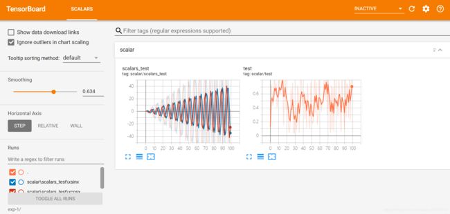
   writer.add_scalar('scalar/test', np.random.rand(), epoch)
   writer.add_scalars('scalar/scalars_test', {'xsinx': epoch * np.sin(epoch), 'xcosx': epoch * np.cos(epoch)}, epoch)

writer.close()

效果如图所示：

注：可以使用左下角的文件选择你想显示的某个或者全部图片

Add image

An image is represented as 3-dimensional tensor of size [3, H, W].

writer.add_image('imresult', x, iteration)

If you have a batch of images to show, use torchvision’s make_grid function to prepare the image array and send the result to add_image(...) (make_grid takes a 4D tensor and returns tiled images in 3D tensor).

Remember to normalize your image.

Add histogram

Saving histograms is expensive. Both in computation time and storage. If training slows down after using this package, check this first.

To save a histogram, convert the array into numpy array and save with

writer.add_histogram('hist', array, iteration)

Add figure

You can save a matplotlib figure to tensorboard with the add_figure function.

figure input should be matplotlib.pyplot.figure or a list of matplotlib.pyplot.figure.

add_figure('figure', figure, iteration)

Add graph

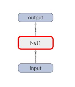
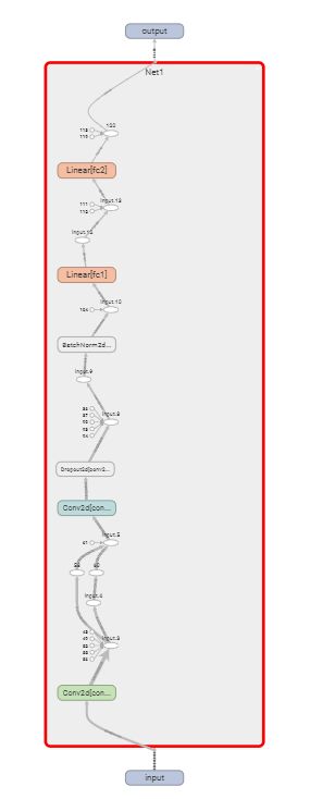
To visualize a model, you need a model m and the input t. t can be a tensor or a list of tensors depending on your model. If error happens, make sure that m(t) runs without problem first.

The graph demo

import torch
import torch.nn as nn
import torch.nn.functional as F
from tensorboardX import SummaryWriter


class Net1(nn.Module):
    def __init__(self):
        super(Net1, self).__init__()
        self.conv1 = nn.Conv2d(1, 10, kernel_size=5)
        self.conv2 = nn.Conv2d(10, 20, kernel_size=5)
        self.conv2_drop = nn.Dropout2d()
        self.fc1 = nn.Linear(320, 50)
        self.fc2 = nn.Linear(50, 10)
        self.bn = nn.BatchNorm2d(20)

    def forward(self, x):
        x = F.max_pool2d(self.conv1(x), 2)
        x = F.relu(x) + F.relu(-x)
        x = F.relu(F.max_pool2d(self.conv2_drop(self.conv2(x)), 2))
        x = self.bn(x)
        x = x.view(-1, 320)
        x = F.relu(self.fc1(x))
        x = F.dropout(x, training=self.training)
        x = self.fc2(x)
        x = F.softmax(x, dim=1)
        return x


dummy_input = torch.rand(13, 1, 28, 28)

model = Net1()
# with语句，可以避免因w.close()未写造成的问题
with SummaryWriter(comment='Net1') as w:
    w.add_graph(model, (dummy_input,))

这里有个比较坑的地方，如果使用的pytorch版本大于1.3.1，那graph是显示不出来的，有两种解决方案，第一种比较粗暴，就是直接卸载高版本的pytorch后再装一个低版本的。第二种是直接用tensorboard，只要把代码中的from tensorboardX import SummaryWriter替换成from torch.utils.tensorboard import SummaryWriter即可！

成功显示网络结构：

双击方框查看网络细节：

Add audio

add_audio(tag, audio, iteration, sample_rate)

audio is an one dimensional array, and each element in the array represents the consecutive amplitude samples. For a 2 seconds audio with sample_rate 44100 Hz, the input x should have 88200 elements. Each element should lie in [−1, 1].

Add embedding(高维度张量可视化/降维)

Embeddings, high dimensional data, can be visualized and converted into human perceptible 3D data by tensorboard, which provides PCA and t-sne to project the data into low dimensional space.

What you need to do is provide a bunch of points and tensorboard will do the rest for you. The bunch of points is passed as a tensor of size n x d, where n is the number of points and d is the feature dimension. The feature representation can either be raw data (e.g. the MNIST image) or a representation learned by your network (extracted feature). This determines how the points distributes.

To make the visualization more informative, you can pass optional metadata or label_imgs for each data points. In this way you can see that neighboring point have similar label and distant points have very different label (semantically or visually). Here the metadata is a list of labels, and the length of the list should equal to n, the number of the points. The label_imgs is a 4D tensor of size NCHW. N should equal to n as well.

The embedding demo

查看数据可视化效果

tensorboard --logdir="runs/exp-1/"

在浏览器中输入http://localhost:6006/即可

官方demo

import torch
import torchvision.utils as vutils
import numpy as np
import torchvision.models as models
from torchvision import datasets
from tensorboardX import SummaryWriter

resnet18 = models.resnet18(False)
writer = SummaryWriter()
sample_rate = 44100
freqs = [262, 294, 330, 349, 392, 440, 440, 440, 440, 440, 440]

for n_iter in range(100):

    dummy_s1 = torch.rand(1)
    dummy_s2 = torch.rand(1)
    # data grouping by `slash`
    writer.add_scalar('data/scalar1', dummy_s1[0], n_iter)
    writer.add_scalar('data/scalar2', dummy_s2[0], n_iter)

    writer.add_scalars('data/scalar_group', {'xsinx': n_iter * np.sin(n_iter),
                                             'xcosx': n_iter * np.cos(n_iter),
                                             'arctanx': np.arctan(n_iter)}, n_iter)

    dummy_img = torch.rand(32, 3, 64, 64)  # output from network
    if n_iter % 10 == 0:
        x = vutils.make_grid(dummy_img, normalize=True, scale_each=True)
        writer.add_image('Image', x, n_iter)

        dummy_audio = torch.zeros(sample_rate * 2)
        for i in range(x.size(0)):
            # amplitude of sound should in [-1, 1]
            dummy_audio[i] = np.cos(freqs[n_iter // 10] * np.pi * float(i) / float(sample_rate))
        writer.add_audio('myAudio', dummy_audio, n_iter, sample_rate=sample_rate)

        writer.add_text('Text', 'text logged at step:' + str(n_iter), n_iter)

        for name, param in resnet18.named_parameters():
            writer.add_histogram(name, param.clone().cpu().data.numpy(), n_iter)

        # needs tensorboard 0.4RC or later
        writer.add_pr_curve('xoxo', np.random.randint(2, size=100), np.random.rand(100), n_iter)

dataset = datasets.MNIST('mnist', train=False, download=True)
images = dataset.test_data[:100].float()
label = dataset.test_labels[:100]

features = images.view(100, 784)
writer.add_embedding(features, metadata=label, label_img=images.unsqueeze(1))

# export scalar data to JSON for external processing
writer.export_scalars_to_json("./all_scalars.json")
writer.close()

示例：可视化loss及graph

import torch
import torch.nn as nn
from tensorboardX import SummaryWriter
import matplotlib.pyplot as plt
import numpy as np

input_size = 1
output_size = 1
num_epoches = 60
learning_rate = 0.01
writer = SummaryWriter(comment='Linear')
x_train = np.array([[3.3], [4.4], [5.5], [6.71], [6.93], [4.168],
                    [9.779], [6.182], [7.59], [2.167], [7.042],
                    [10.791], [5.313], [7.997], [3.1]], dtype=np.float32)
y_train = np.array([[1.7], [2.76], [2.09], [3.19], [1.694], [1.573],
                    [3.366], [2.596], [2.53], [1.221], [2.827],
                    [3.465], [1.65], [2.904], [1.3]], dtype=np.float32)

model = nn.Linear(input_size, output_size)

criterion = nn.MSELoss()
optimizer = torch.optim.SGD(model.parameters(), lr=learning_rate)

for epoch in range(num_epoches):
    inputs = torch.from_numpy(x_train)
    targets = torch.from_numpy(y_train)

    output = model(inputs)
    loss = criterion(output, targets)

    optimizer.zero_grad()
    loss.backward()
    optimizer.step()
    # 保存loss的数据与epoch数值
    writer.add_scalar('Train', loss, epoch)
    if (epoch + 1) % 5 == 0:
        print('Epoch {}/{},loss:{:.4f}'.format(epoch + 1, num_epoches, loss.item()))

# 将model保存为graph
writer.add_graph(model, (inputs,))

predicted = model(torch.from_numpy(x_train)).detach().numpy()
plt.plot(x_train, y_train, 'ro', label='Original data')
plt.plot(x_train, predicted, label='Fitted line')
plt.legend()
plt.show()
writer.close()

Visdom

Github：https://github.com/facebookresearch/visdom
本节参考：https://www.cnblogs.com/fanghao/p/10256287.html
https://blog.csdn.net/wen_fei/article/details/82979497
https://blog.csdn.net/u012436149/article/details/69389610

Visdom支持torch和numpy，目的是促进远程数据的可视化

安装

conda install jsonpatch
conda install visdom

启动服务

python -m visdom.server # visdom服务是一个Web Server服务，默认端口为8097，可以根据需要加上-p选项修改端口

The visdom command is equivalent to running python -m visdom.server.

If the above does not work, try using an SSH tunnel to your server by adding the following line to your local ~/.ssh/config: LocalForward 127.0.0.1:8097 127.0.0.1:8097.

The following options can be provided to the server:

• port : The port to run the server on.
• hostname : The hostname to run the server on.
• base_url : The base server url (default = /).
• env_path : The path to the serialized session to reload.
• logging_level : Logging level (default = INFO). Accepts both standard text and numeric logging values.
• readonly : Flag to start server in readonly mode.
• enable_login : Flag to setup authentication for the sever, requiring a username and password to login.
• force_new_cookie : Flag to reset the secure cookie used by the server, invalidating current login cookies. Requires -enable_login.

When -enable_login flag is provided, the server asks user to input credentials using terminal prompt. Alternatively, you can setup VISDOM_USE_ENV_CREDENTIALS env variable, and then provide your username and password via VISDOM_USERNAME and VISDOM_PASSWORD env variables without manually interacting with the terminal. This setup is useful in case if you would like to launch visdom server from bash script, or from Jupyter notebook.

VISDOM_USERNAME=username
VISDOM_PASSWORD=password
VISDOM_USE_ENV_CREDENTIALS=1 visdom -enable_login

You can also use VISDOM_COOKIE variable to provide cookies value if the cookie file wasn’t generated, or the flag -force_new_cookie was set.

可能会遇到卡死的问题，原因是下载一些js、css资源文件比较慢或者根本没法访问，解决方案是手动下载即可。在D:\Software\Anaconda3\envs\pytorch\Lib\site-packages\visdom\server.py中找到download_scripts()，手动下载资源文件即可

D:\Software\Anaconda3\envs\pytorch\Lib\site-packages\visdom\为install_dir

链接	保存地址
https://unpkg.com/[email protected]/dist/jquery.min.js	install_dir/static/js/jquery.min.js
https://unpkg.com/[email protected]/dist/js/bootstrap.min.js	install_dir/static/js/bootstrap.min.js
https://unpkg.com/[email protected]/umd/react.production.min.js	install_dir/static/js/react-react.min.js
https://unpkg.com/[email protected]/umd/react-dom.production.min.js	install_dir/static/js/react-dom.min.js
https://unpkg.com/[email protected]/dist/react-modal.min.js	install_dir/static/js/react-modal.min.js
https://cdnjs.cloudflare.com/ajax/libs/mathjax/2.7.1/MathJax.js?config=TeX-AMS-MML_SVG	install_dir/static/js/mathjax-MathJax.js
https://cdn.plot.ly/plotly-latest.min.js	install_dir/static/js/plotly-plotly.min.js
https://unpkg.com/[email protected]/sjcl.js	install_dir/static/js/sjcl.js
https://unpkg.com/[email protected]/css/styles.css	install_dir/static/css/react-resizable-styles.css
https://unpkg.com/[email protected]/css/styles.css	install_dir/static/css/react-grid-layout-styles.css
https://unpkg.com/[email protected]/dist/css/bootstrap.min.css	install_dir/static/css/bootstrap.min.css
https://unpkg.com/[email protected]	install_dir/static/fonts/classnames
https://unpkg.com/[email protected]/dist/layout-bin-packer.js	install_dir/static/js/layout_bin_packer.js
https://unpkg.com/[email protected]/dist/fonts/glyphicons-halflings-regular.eot	install_dir/static/fonts/glyphicons-halflings-regular.eot
https://unpkg.com/[email protected]/dist/fonts/glyphicons-halflings-regular.woff2	install_dir/static/fonts/glyphicons-halflings-regular.woff2
https://unpkg.com/[email protected]/dist/fonts/glyphicons-halflings-regular.woff	install_dir/static/fonts/glyphicons-halflings-regular.woff
https://unpkg.com/[email protected]/dist/fonts/glyphicons-halflings-regular.ttf	install_dir/static/fonts/glyphicons-halflings-regular.ttf
https://unpkg.com/[email protected]/dist/fonts/glyphicons-halflings-regular.svg#glyphicons_halflingsregular	install_dir/static/fonts/glyphicons-halflings-regular.svg#glyphicons_halflingsregular

看文件夹里缺哪个就下哪个吧
后来又在网上看到有上传好的static文件夹，直接解压到install_dir/目录下即可：https://blog.csdn.net/qq_32523711/article/details/103345741

在启动服务时我还碰到了一个问题：

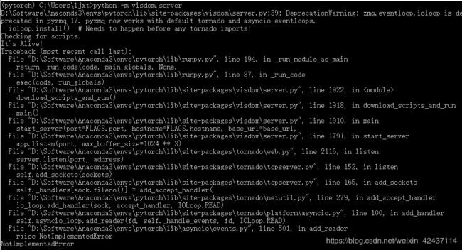
解决方法：
参考：https://blog.csdn.net/B1151937289/article/details/106169017/

添加下面两行代码到D:\Software\Anaconda3\envs\pytorch\Lib\site-packages\visdom\server.py的相应位置即可：

import asyncio
asyncio.set_event_loop_policy(asyncio.WindowsSelectorEventLoopPolicy())

修改后启动服务成功：

启动服务后，在浏览器中输入http://localhost:8097来访问 Visdom

基本概念

Windows / Panes(窗格)

UI刚开始是个白板–您可以用图像，图片，文本填充它。这些填充的数据出现在 Panes 中，您可以这些Panes进行 拖放，删除，调整大小和销毁操作。Panes是保存在 envs 中的， envs的状态存储在会话之间。您可以下载Panes中的内容–包括您在svg中的绘图。

Tip: You can use the zoom of your browser to adjust the scale of the UI.

Callbacks

The python Visdom implementation supports callbacks on a window. The functionality of these callbacks allows the Visdom object to receive and react to events that happen in the frontend.

You can subscribe a window to events by adding a function to the event handlers dict for the window id you want to subscribe by calling viz.register_event_handler(handler, win_id) with your handler and the window id. Multiple handlers can be registered to the same window. You can remove all event handlers from a window using viz.clear_event_handlers(win_id). When an event occurs to that window, your callbacks will be called on a dict containing:

• event_type: one of the below event types
• pane_data: all of the stored contents for that window including layout and content.
• eid: the current environment id
• target: the window id the event is called on

Right now the following callback events are supported:

• Close - Triggers when a window is closed. Returns a dict with only the aforementioned fields.
• KeyPress - Triggers when a key is pressed. Contains additional parameters:
  key - A string representation of the key pressed (applying state modifiers such as SHIFT)
  key_code - The javascript event keycode for the pressed key (no modifiers)
• PropertyUpdate - Triggers when a property is updated in Property pane
  propertyId - Position in properties list
  value - New property value
• Click - Triggers when Image pane is clicked on, has a parameter:
  image_coord - dictionary with the fields x and y for the click coordinates in the coordinate frame of the possibly zoomed/panned image (not the enclosing pane).

import visdom

# 创建visdom客户端，环境为first
vis = visdom.Visdom(env='first')

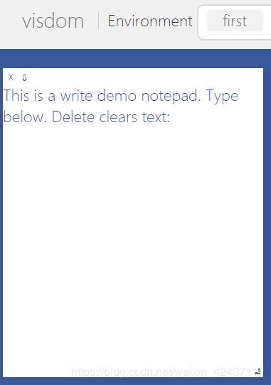
txt = 'This is a write demo notepad. Type below. Delete clears text:
'
callback_text_window = vis.text(txt, win='callback')

def type_callback(event):
    if event['event_type'] == 'KeyPress':
        curr_txt = event['pane_data']['content']
        if event['key'] == 'Enter':
            curr_txt += '
'
        elif event['key'] == 'Backspace':
            curr_txt = curr_txt[:-1]
        elif event['key'] == 'Delete':
            curr_txt = txt
        elif len(event['key']) == 1:
            curr_txt += event['key']
        vis.text(curr_txt, win=callback_text_window)

vis.register_event_handler(type_callback, callback_text_window)

Environments(环境)

您可以使用envs对可视化空间进行分区。默认地，每个用户都会有一个叫做main的envs。可以通过编程或UI创建新的envs。envs的状态是长期保存的。

可以通过 url: http://localhost.com:8097/env/main 访问特定的env

Comparing Environments

Selecting multiple environments in the check box will query the server for the plots with the same titles in all environments and plot them in a single plot. An additional compare legend pane is created with a number corresponding to each selected environment. Individual plots are updated with legends corresponding to “x_name” where x is a number corresponding with the compare legend pane and name is the original name in the legend.

Note: The compare envs view is not robust to high throughput data, as the server is responsible for generating the compared content. Do not compare an environment that is receiving a high quantity of updates on any plot, as every update will request regenerating the comparison. If you need to compare two plots that are receiving high quantities of data, have them share the same window on a singular env.

Managing Environments

Pressing the folder icon opens a dialog that allows you to fork or force save the current environment, or delete any of your existing environments.

Env Files: Your envs are loaded at initialization of the server, by default from $HOME/.visdom/. Custom paths can be passed as a cmd-line argument. Envs are removed by using the delete button or by deleting the corresponding .json file from the env dir.

State

Once you’ve created a few visualizations, state is maintained. The server automatically caches your visualizations – if you reload the page, your visualizations reappear.

• Save: You can manually do so with the save button. This will serialize the env’s state (to disk, in JSON), including window positions. You can save an env programmatically.

• Fork: If you enter a new env name, saving will create a new env – effectively forking the previous env.

Filter

You can use the filter to dynamically sift through windows present in an env – just provide a regular expression with which to match titles of window you want to show.

Views

It is possible to manage the views simply by dragging the tops of windows around, however additional features exist to keep views organized and save common views.

Saving/Deleting Views

Using the folder icon, a dialog window opens where views can be forked in the same way that envs can be. Saving a view will retain the position and sizes of all of the windows in a given environment. Views are saved in $HOME/.visdom/view/layouts.json in the visdom filepath.

Re-Packing

Using the repack icon (9 boxes), visdom will attempt to pack your windows in a way that they best fit while retaining row/column ordering.

Reloading Views

实验

注意：在使用时不能将源文件命名为visdom.py，否则代码内调包会优先调用当前文件夹内的文件，导致报错

可以参考的实验

https://www.cnblogs.com/fanghao/p/10256287.html

官方demo

https://github.com/facebookresearch/visdom/tree/master/example

API

大多数API的输入包含，一个tensor X（保存数据）和一个可选的tensor Y（保存标签或者时间戳）。所有的绘图函数都接收一个可选参数win，用来将图画到一个特定的window(pane)上。每个绘图函数也会返回当前绘图的win。您也可以指定将图添加到哪个env上。

画图的方法的接口一般是 vis.some_func(X,Y, opts={})
opts存放当前pane的一些简单设置，下面的是比较通用的一些配置
options.title，options.xlabel，options.ylabel

如果想在同一个图中画多个曲线，加上update="append"参数即可

Basics

• vis.image : image
• vis.images : list of images
• vis.text : arbitrary HTML
• vis.properties : properties grid
• vis.audio : audio
• vis.video : videos
• vis.svg : SVG object
• vis.matplot : matplotlib plot
• vis.save : serialize state server-side

vis.image

It takes as input an CxHxW tensor img that contains the image.

The following opts are supported:

• jpgquality: JPG quality (number 0-100). If defined image will be saved as JPG to reduce file size. If not defined image will be saved as PNG.
• caption: Caption for the image
• store_history: Keep all images stored to the same window and attach a slider to the bottom that will let you select the image to view. You must always provide this opt when sending new images to an image with history.

Note You can use alt on an image pane to view the x/y coordinates of the cursor. You can also ctrl-scroll to zoom, alt scroll to pan vertically, and alt-shift scroll to pan horizontally. Double click inside the pane to restore the image to default.

import visdom
import torch

# 创建visdom客户端，环境为first
vis = visdom.Visdom(env='first')

vis.image(torch.randn(3, 256, 256), win='random_image')

vis.images

It takes an input B x C x H x W tensor or a list of images all of the same size. It makes a grid of images of size (B / nrow, nrow).

The following arguments and opts are supported:

• nrow: Number of images in a row
• padding: Padding around the image, equal padding around all 4 sides
• opts.jpgquality: JPG quality (number 0-100). If defined image will be saved as JPG to reduce file size. If not defined image will be saved as PNG.
• opts.caption: Caption for the image

import visdom
import torch

# 创建visdom客户端，环境为first
vis = visdom.Visdom(env='first')

vis.images(
    torch.randn(20, 3, 64, 64),
    opts=dict(title='Random images', caption='How random.'))

vis.text

It takes as input a text string. No specific opts are currently supported.

import visdom

# 创建visdom客户端，环境为first
vis = visdom.Visdom(env='first')

# win参数表示显示的窗格(pane)名字
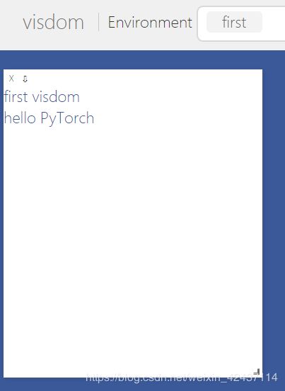
vis.text('first visdom', win='text1')
# 使用 append=True 来增加text，否则会覆盖之前的text
vis.text('hello PyTorch', win='text1', append=True)

vis.video

It takes as input the filename of the video videofile or a LxHxWxC-sized tensor containing all the frames of the video as input. The function does not support any plot-specific opts.

The following opts are supported:

• opts.fps: FPS for the video (integer > 0; default = 25)

Note: Using tensor input requires that ffmpeg and cv2 is installed and working. Your ability to play video may depend on the browser you use: your browser has to support the Theano codec in an OGG container (Chrome supports this).

import visdom
import numpy as np

# 创建visdom客户端，环境为first
vis = visdom.Visdom(env='first')

video = np.empty([256, 250, 250, 3], dtype=np.uint8)
for n in range(256):
    video[n, :, :, :].fill(n)
vis.video(tensor=video)

这里用tensor显示video报错，没用过opencv，等以后再解决吧

D:\Software\Anaconda3\envs\pytorch\lib\site-packages\visdom\__init__.py in video(self, tensor, dim, videofile, win, env, opts)
   1406                 (tensor.shape[2], tensor.shape[1])
   1407             )
-> 1408             assert writer.isOpened(), 'video writer could not be opened'
   1409             for i in range(tensor.shape[0]):
   1410                 # TODO mute opencv on this function call somehow

AssertionError: video writer could not be opened

import visdom

# 创建visdom客户端，环境为first
vis = visdom.Visdom(env='first')

vis.video(videofile='E:/Workspace/python/jupyter/pytorch/trailer.ogv', 
			opts={'width': 864, 'height': 480})

vis.matplot

This function draws a Matplotlib plot. The function supports one plot-specific option: resizable.

Note When set to True the plot is resized with the pane. You need beautifulsoup4 and lxml packages installed to use this option.

Note: matplot is not rendered using the same backend as plotly plots, and is somewhat less efficient. Using too many matplot windows may degrade visdom performance.

import visdom
import matplotlib.pyplot as plt

# 创建visdom客户端，环境为first
vis = visdom.Visdom(env='first')

plt.plot([1, 23, 2, 4])
plt.ylabel('some numbers')
vis.matplot(plt)

Plotting

• vis.scatter : 2D or 3D scatter plots
• vis.line : line plots
• vis.stem : stem plots 茎叶图
• vis.heatmap : heatmap plots
• vis.bar : bar graphs 条形图
• vis.histogram : histograms 直方图
• vis.boxplot : boxplots 箱型图
• vis.surf : surface plots 表面图
• vis.contour : contour plots 轮廓图
• vis.quiver : quiver plots 绘出二维矢量场
• vis.mesh : mesh plots 网格图
• vis.dual_axis_lines : double y axis line plots

vis.scatter

This function draws a 2D or 3D scatter plot. It takes as input an Nx2 or Nx3 tensor X that specifies the locations of the N points in the scatter plot. An optional N tensor Y containing discrete labels that range between 1 and K can be specified as well – the labels will be reflected in the colors of the markers.

update can be used to efficiently update the data of an existing plot. Use ’append' to append data, ’replace' to use new data, or ’remove' to remove the trace specified by name. Using update='append' will create a plot if it doesn’t exist and append to the existing plot otherwise. If updating a single trace, use name to specify the name of the trace to be updated. Update data that is all NaN is ignored (can be used for masking update).

The following opts are supported:

• opts.markersymbol : marker symbol 标记符号 (string; default = 'dot')
• opts.markersize : marker size (number; default = '10')
• opts.markercolor : color per marker. (torch.*Tensor; default = nil)
• opts.markerborderwidth: marker border line width (float; default = 0.5)
• opts.legend : table containing legend names
• opts.textlabels : text label for each point (list: default = None)
• opts.layoutopts : dict of any additional options that the graph backend accepts for a layout. For example layoutopts = {'plotly': {'legend': {'x':0, 'y':0}}}.
• opts.traceopts : dict mapping trace names or indices to dicts of additional options that the graph backend accepts. For example traceopts = {'plotly': {'myTrace': {'mode': 'markers'}}}.
• opts.webgl : use WebGL for plotting (boolean; default = false). It is faster if a plot contains too many points. Use sparingly as browsers won’t allow more than a couple of WebGL contexts on a single page.

opts.markercolor is a Tensor with Integer values. The tensor can be of size N or N x 3 or K or K x 3.

• Tensor of size N: Single intensity value per data point. 表示每个点的单通道颜色强度 0 = black, 255 = red
• Tensor of size N x 3: Red, Green and Blue intensities per data point. 0,0,0 = black, 255,255,255 = white
• Tensor of size K and K x 3: Instead of having a unique color per data point, the same color is shared for all points of a particular label.

import visdom
import torch

# 创建visdom客户端，环境为first
vis = visdom.Visdom(env='first')

Y = torch.rand(100)
    
win=vis.scatter(
    X=torch.rand(100, 2),
    Y=(Y[Y > 0] + 1.5).int(),
    opts=dict(
        legend=['Apples', 'Pears'],
        xtickmin=0,
        xtickmax=1,
        xtickstep=0.5,
        ytickmin=0,
        ytickmax=1,
        ytickstep=0.5,
        markersymbol='cross-thin-open',
    ),
)

# add new trace to scatter plot
vis.scatter(
    X=torch.rand(255),
    Y=torch.rand(255),
    win=win,
    opts=dict(
        markersymbol='cross-thin-open'
    ), 
    name='new_trace',
    update='append'
)

vis.scatter(
    X=torch.rand(100, 3),
    Y=(Y + 1.5).int(),
    opts=dict(
        legend=['Men', 'Women'],
        markersize=5,
        xtickmin=0,
        xtickmax=2,
        xlabel='Arbitrary',
        xtickvals=[0, 0.75, 1.6, 2],
        ytickmin=0,
        ytickmax=2,
        ytickstep=0.5,
        ztickmin=0,
        ztickmax=1,
        ztickstep=0.5,
    )
)

vis.line

This function draws a line plot. It takes as input an N or NxM tensor Y that specifies the values of the M lines (that connect N points) to plot. It also takes an optional X tensor that specifies the corresponding x-axis values; X can be an N tensor (in which case all lines will share the same x-axis values) or have the same size as Y.

update can be used to efficiently update the data of an existing plot. Use ‘append’ to append data, ‘replace’ to use new data, or ‘remove’ to remove the trace specified by name. If updating a single trace, use name to specify the name of the trace to be updated. Update data that is all NaN is ignored (can be used for masking update).

The following opts are supported:

• opts.fillarea : fill area below line (boolean)
• opts.markers : show markers (boolean; default = false)
• opts.markersymbol: marker symbol (string; default = 'dot')
• opts.markersize : marker size (number; default = '10')
• opts.linecolor : line colors (np.array; default = None)
• opts.dash : line dash type for each line (np.array; default = 'solid'), one of solid, dash, dashdot , size should match number of lines being drawn
• opts.legend : table containing legend names
• opts.layoutopts : dict of any additional options that the graph backend accepts for a layout. For example layoutopts = {'plotly': {'legend': {'x':0, 'y':0}}}.
• opts.traceopts : dict mapping trace names or indices to dicts of additional options that plot.ly accepts for a trace.
• opts.webgl : use WebGL for plotting (boolean; default = false). It is faster if a plot contains too many points. Use sparingly as browsers won’t allow more than a couple of WebGL contexts on a single page.

import visdom
import numpy as np

# 创建visdom客户端，环境为first
vis = visdom.Visdom(env='first')

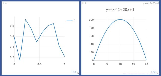
vis.line(Y=np.random.rand(10), opts=dict(showlegend=True))


# 绘制 y=-x^2+20x+1，opts可以进行标题、坐标轴标签等配置
x = torch.arange(21)
y = -x**2 + 20 * x + 1
vis.line(X=x, Y=y, opts={'title': 'y=-x^2+20x+1'}, win='loss')

Generic Plots

Note that the server API adheres to the Plotly convention of data and layout objects, such that you can produce your own arbitrary Plotly visualizations:

import visdom
vis = visdom.Visdom()

trace = dict(x=[1, 2, 3], y=[4, 5, 6], mode="markers+lines", type='custom',
             marker={'color': 'red', 'symbol': 104, 'size': "10"},
             text=["one", "two", "three"], name='1st Trace')
layout = dict(title="First Plot", xaxis={'title': 'x1'}, yaxis={'title': 'x2'})

vis._send({'data': [trace], 'layout': layout, 'win': 'mywin'})

Customizing plots

绘图函数使用可选的options表作为输入。用它来修改默认的绘图属性。所有输入参数在单个表中指定;输入参数是基于输入表中键的匹配。

下列的选项除了对于vis.image, vis.text, vis.video, vis.audio不可用以外，其他的绘图函数都适用。我们称为通用选项。

• opts.title : figure title
• opts.width : figure width
• opts.height : figure height
• opts.showlegend : show legend (true or false)
• opts.xtype : type of x-axis ('linear' or 'log')
• opts.xlabel : label of x-axis
• opts.xtick : show ticks on x-axis (boolean)
• opts.xtickmin : first tick on x-axis (number)
• opts.xtickmax : last tick on x-axis (number)
• opts.xtickstep : distances between ticks on x-axis (number)
• opts.ytype : type of y-axis ('linear' or 'log')
• opts.ylabel : label of y-axis
• opts.ytick : show ticks on y-axis (boolean)
• opts.ytickmin : first tick on y-axis (number)
• opts.ytickmax : last tick on y-axis (number)
• opts.ytickstep : distances between ticks on y-axis (number)
• opts.marginleft : left margin (in pixels)
• opts.marginright : right margin (in pixels)
• opts.margintop : top margin (in pixels)
• opts.marginbottom: bottom margin (in pixels)
  其它的一些选项就是函数特定的选项，在上面API介绍的时候已经提到过。

Others

• vis.close : close a window by id
• vis.delete_env : delete an environment by env_id
• vis.win_exists : check if a window already exists by id
• vis.get_env_list : get a list of all of the environments on your server
• vis.win_hash: get md5 hash of window’s contents
• vis.get_window_data: get current data for a window
• vis.check_connection: check if the server is connected
• vis.replay_log: replay the actions from the provided log file

vis.stem

这个函数用来画茎叶图。它需要一个形状为N或者N*M的 tensor X 来指定M时间序列中N个点的值。一个可选择的Y，形状为N或者N×M，用Y来指定时间戳，如果Y的形状是N，那么默认M时间序列共享同一个时间戳。

支持以下特定选项：

• options.colormap : 色图 (string; default = 'Viridis')
• options.legend : 保存图例名字的 table

vis.heatmap

这个函数用来画热力图。它输入一个 形状为N×M的 tensor X。X指定了热力图中位置的值。

支持下列特定选项：

• options.colormap : 色图 (string; default = 'Viridis')
• options.xmin : 小于这个值的会被剪切成这个值(number; default = X:min())
• options.xmax : 大于这个值的会被剪切成这个值 (number; default = X:max())
• options.columnnames: 包含x轴标签的table
• options.rownames : 包含y轴标签的table

vis.bar

这个函数可以画正常的，堆起来的，或分组的的条形图。

输入参数：

• X(tensor):形状 N 或 N×M，指定每个条的高度。如果X有M列，那么每行的值可以看作一组或者把他们值堆起来（取决与options.stacked是否为True）。
• Y(tensor, optional):形状 N，指定对应的x轴的值。

支持以下特定选项：

• options.columnnames: table containing x-axis labels
• options.stacked : stack multiple columns in X
• options.legend : table containing legend labels

vis.histogram

这个函数用来画指定数据的直方图。他需要输入长度为 N 的 tensor X。X保存了构建直方图的值。

支持下面特定选项：

• options.numbins: bins的个数 (number; default = 30)

vis.boxplot

这个函数用来画箱型图：

输入：

• X(tensor): 形状 N或N×M，指定做第m个箱型图的N个值。

支持以下特定选项：

• options.legend: labels for each of the columns in X

vis.surf

这个函数用来画表面图：

输入：

• X(tensor):形状 N×M，指定表面图上位置的值.

支持以下特定选项：

• options.colormap: colormap (string; default = 'Viridis')
• options.xmin : clip minimum value (number; default = X:min())
• options.xmax : clip maximum value (number; default = X:max())

vis.contour

这个函数用来画轮廓图。

输入：

• X(tensor)：形状 N×M，指定了轮廓图中的值

支持以下特定选项：

• options.colormap: colormap (string; default = 'Viridis')
• options.xmin : clip minimum value (number; default = X:min())
• options.xmax : clip maximum value (number; default = X:max())

vis.quiver

这个函数用来画二维矢量场图。

输入：

• X(tensor): 形状 N*M
• Y(tensor):形状 N*M
• gridX(tensor, optional):形状 N*M
• gradY(tensor, optional): 形状 N*M
X 与 Y决定了 箭头的长度和方向。可选的gridX和gridY指定了偏移。

支持下列特定选项：

• options.normalize: 最长肩头的长度 (number)
• options.arrowheads: 是否现实箭头 (boolean; default = true)

vis.svg

此函数绘制一个SVG对象。输入是一个SVG字符串或 一个SVG文件的名称。该功能不支持任何特定的功能options。

vis.mesh

此函数画出一个网格图。

输入：

• X(tensor): shape(N*2或N*3) 定义N个顶点
• Y(tensor， optional)：shape(M*2或M×3) 定义多边形

支持下列特定选项:

• options.color: color (string)
• options.opacity: 多边形的不透明性 (number between 0 and 1)