HOW POWERFUL ARE GRAPH NEURAL NETWORKS?

HOW POWERFUL ARE GRAPH NEURAL NETWORKS?

ABSTRACT

Graph Neural Networks (GNNs) are an effective framework for representation learning of graphs. GNNs follow a neighborhood aggregation scheme, where the representation vector of a node is computed by recursively aggregating and trans-forming representation vectors of its neighboring nodes. Many GNN variants have been proposed and have achieved state-of-the-art results on both node and graph classification tasks. However, despite GNNs revolutionizing graph representation learning, there is limited understanding of their representational properties and limitations. Here, we present a theoretical framework for analyzing the expressive power of GNNs to capture different graph structures. Our results characterize the discriminative power of popular GNN variants, such as Graph Convolutional Networks and GraphSAGE, and show that they cannot learn to distinguish certain simple graph structures. We then develop a simple architecture that is provably the most expressive among the class of GNNs and is as powerful as the Weisfeiler-Lehman graph isomorphism test. We empirically validate our theoretical findings on a number of graph classification benchmarks, and demonstrate that our model achieves state-of-the-art performance.
图神经网络（GNN）是图表表示学习的有效框架。 GNN遵循邻域聚合方案，其中节点的表示向量通过递归地聚合和变换其相邻节点的表示向量来计算。已经提出了许多GNN变体，并且已经在节点和图形分类任务上获得了最先进的结果。然而，尽管GNN改变了图形表示学习，但对其表示属性和局限性的理解有限。在这里，我们提出了一个理论框架，用于分析GNN的表达能力，以捕获不同的图形结构。我们的结果表征了流行的GNN变体（如图形卷积网络和GraphSAGE）的判别力，并表明它们无法学会区分某些简单的图形结构。然后，我们开发了一个简单的体系结构，它可以证明是GNN类中最具表现力的体系，并且与Weisfeiler-Lehman图同构测试一样强大。我们在许多图表分类基准测试中凭经验验证了我们的理论发现，并证明我们的模型实现了最先进的性能。

1 INTRODUCTION

Learning with graph structured data, such as molecules, social, biological, and financial networks, requires effective representation of their graph structure (Hamilton et al., 2017b). Recently, there has been a surge of interest in Graph Neural Network (GNN) approaches for representation learning of graphs (Li et al., 2016; Hamilton et al., 2017a; Kipf & Welling, 2017; Velickovic et al., 2018; Xu et al., 2018). GNNs broadly follow a recursive neighborhood aggregation (or message passing) scheme, where each node aggregates feature vectors of its neighbors to compute its new feature vector (Xu et al., 2018; Gilmer et al., 2017). After k iterations of aggregation, a node is represented by its transformed feature vector, which captures the structural information within the node’s k-hop neighborhood. The representation of an entire graph can then be obtained through pooling (Ying et al., 2018), for example, by summing the representation vectors of all nodes in the graph.

Many GNN variants with different neighborhood aggregation and graph-level pooling schemes have been proposed (Scarselli et al., 2009b; Battaglia et al., 2016; Defferrard et al., 2016; Duvenaud et al., 2015; Hamilton et al., 2017a; Kearnes et al., 2016; Kipf & Welling, 2017; Li et al., 2016; Velickovic et al., 2018; Santoro et al., 2017; Xu et al., 2018; Santoro et al., 2018; Verma & Zhang, 2018; Ying et al., 2018; Zhang et al., 2018). Empirically, these GNNs have achieved state-of-the-art performance in many tasks such as node classification, link prediction, and graph classification. However, the design of new GNNs is mostly based on empirical intuition, heuristics, and experimental trial-and-error. There is little theoretical understanding of the properties and limitations of GNNs, and formal analysis of GNNs’ representational capacity is limited.

Here, we present a theoretical framework for analyzing the representational power of GNNs. We formally characterize how expressive different GNN variants are in learning to represent and distin-guish between different graph structures. Our framework is inspired by the close connection between GNNs and the Weisfeiler-Lehman (WL) graph isomorphism test (Weisfeiler & Lehman, 1968), a powerful test known to distinguish a broad class of graphs (Babai & Kucera, 1979). Similar to GNNs, the WL test iteratively updates a given node’s feature vector by aggregating feature vectors of its network neighbors. What makes the WL test so powerful is its injective aggregation update that maps different node neighborhoods to different feature vectors. Our key insight is that a GNN can have as large discriminative power as the WL test if the GNN’s aggregation scheme is highly expressive and can model injective functions.

To mathematically formalize the above insight, our framework first represents the set of feature vectors of a given node’s neighbors as a multiset, i.e., a set with possibly repeating elements. Then, the neighbor aggregation in GNNs can be thought of as an aggregation function over the multiset. Hence, to have strong representational power, a GNN must be able to aggregate different multisets into different representations. We rigorously study several variants of multiset functions and theoretically characterize their discriminative power, i.e., how well different aggregation functions can distinguish different multisets. The more discriminative the multiset function is, the more powerful the representational power of the underlying GNN.
学习图形结构化数据，如分子，社会，生物和金融网络，需要有效地表示其图形结构（Hamilton等，2017b）。最近，图形表示学习的图形神经网络（GNN）方法引起了人们的兴趣（Li et al。，2016; Hamilton et al。，2017a; Kipf＆Welling，2017; Velickovic et al。，2018; Xu等，2018）。 GNN广泛遵循递归邻域聚合（或消息传递）方案，其中每个节点聚合其邻居的特征向量以计算其新特征向量（Xu等，2018; Gilmer等，2017）。在k次迭代聚合之后，节点由其变换的特征向量表示，其捕获节点的k-hop邻域内的结构信息。然后可以通过汇集（Ying等，2018）获得整个图的表示，例如，通过对图中所有节点的表示向量求和。

已经提出了许多具有不同邻域聚合和图级汇集方案的GNN变体（Scarselli等，2009b; Battaglia等，2016; Defferrard等，2016; Duvenaud等，2015; Hamilton等， 2017a; Kearnes等人，2016; Kipf＆Welling，2017; Li等人，2016; Velickovic等人，2018; Santoro等人，2017; Xu等人，2018; Santoro等人，2018; Verma＆Zhang，2018; Ying等，2018; Zhang等，2018）。根据经验，这些GNN在许多任务中实现了最先进的性能，例如节点分类，链接预测和图分类。然而，新GNN的设计主要基于经验直觉，启发式和实验性反复试验。关于GNN的性质和局限性的理论知识很少，对GNNs表征能力的形式分析是有限的。

在这里，我们提出了一个分析GNN表示能力的理论框架。我们正式地描述了表达不同的GNN变体在学习如何表示和区分不同图形结构之间的表现。我们的框架受到GNN与Weisfeiler-Lehman（WL）图同构测试（Weisfeiler＆Lehman，1968）之间密切​​联系的启发，这是一种强大的测试，可以区分广泛的图形（Babai和Kucera，1979）。与GNN类似，WL测试通过聚合其网络邻居的特征向量来迭代地更新给定节点的特征向量。使WL测试如此强大的原因在于其内射聚合更新将不同的节点邻域映射到不同的特征向量。我们的主要观点是，如果GNN的聚合方案具有高度表达性并且可以模拟内射函数，则GNN可以具有与WL测试一样大的判别力。

为了在数学上形式化上述见解，我们的框架首先将给定节点的邻居的特征向量集表示为多集，即具有可能重复元素的集合。然后，GNN中的邻居聚合可以被认为是多集合上的聚合函数。因此，为了具有强大的表征能力，GNN必须能够将不同的多重集合聚合成不同的表示。我们严格研究多集函数的几种变体，并在理论上表征它们的判别能力，即不同聚合函数如何区分不同的多集合。多集函数越具有判别性，底层GNN的表示能力就越强大。
Our main results are summarized as follows:

1)We show that GNNs are at most as powerful as the WL test in distinguishing graph structures.

2)We establish conditions on the neighbor aggregation and graph readout functions under which the resulting GNN is as powerful as the WL test.

3)We identify graph structures that cannot be distinguished by popular GNN variants, such as GCN (Kipf & Welling, 2017) and GraphSAGE (Hamilton et al., 2017a), and we precisely characterize the kinds of graph structures such GNN-based models can capture.

4)We develop a simple neural architecture, Graph Isomorphism Network (GIN), and show that its discriminative/representational power is equal to the power of the WL test.

We validate our theory via experiments on graph classification datasets, where the expressive power of GNNs is crucial to capture graph structures. In particular, we compare the performance of GNNs with various aggregation functions. Our results confirm that the most powerful GNN by our theory, i.e., Graph Isomorphism Network (GIN), also empirically has high representational power as it almost perfectly fits the training data, whereas the less powerful GNN variants often severely underfit the training data. In addition, the representationally more powerful GNNs outperform the others by test set accuracy and achieve state-of-the-art performance on many graph classification benchmarks.
我们的主要结果总结如下：

1）我们证明GNN在区分图形结构方面最多与WL测试一样强大。

2）我们在邻居聚合和图形读出函数上建立条件，在这些函数下，生成的GNN与WL测试一样强大。

3）我们识别不能通过流行的GNN变体区分的图结构，例如GCN（Kipf＆Welling，2017）和GraphSAGE（Hamilton等，2017a），并且我们精确地表征了诸如基于GNN的模型的图形结构的种类。可以捕捉。

4）我们开发了一个简单的神经结构，图形同构网络（GIN），并表明它的判别/表征能力等于WL测试的功效。

我们通过图分类数据集上的实验来验证我们的理论，其中GNN的表达能力对于捕获图结构至关重要。特别是，我们将GNN的性能与各种聚合函数进行比较。我们的结果证实，我们的理论中最强大的GNN，即图形同构网络（GIN），在经验上也具有很高的代表性能力，因为它几乎完全适合训练数据，而功能较弱的GNN变体通常严重不适合训练数据。此外，代表性更强大的GNN通过测试集精度优于其他GNN，并在许多图分类基准上实现最先进的性能。

2 PRELIMINARIES

We begin by summarizing some of the most common GNN models and, along the way, introduce our notation. Let G = (V; E) denote a graph with node feature vectors Xv for v 2 V . There are two tasks of interest: (1) Node classification, where each node v 2 V has an associated label yv and the goal is to learn a representation vector hv of v such that v’s label can be predicted as yv = f(hv); (2) Graph classification, where, given a set of graphs fG1; :::; GN g G and their labels fy1; :::; yN g Y, we aim to learn a representation vector hG that helps predict the label of an entire graph, yG = g(hG).

Graph Neural Networks. GNNs use the graph structure and node features Xv to learn a representa-tion vector of a node, hv, or the entire graph, hG. Modern GNNs follow a neighborhood aggregation strategy, where we iteratively update the representation of a node by aggregating representations of its neighbors. After k iterations of aggregation, a node’s representation captures the structural information within its k-hop network neighborhood. Formally, the k-th layer of a GNN is
我们首先总结一些最常见的GNN模型，并在此过程中介绍我们的符号。令G =（V; E）表示具有v 2 V的节点特征向量X v的图。有两个感兴趣的任务：（1）节点分类，其中每个节点v 2 V具有关联的标签yv，并且目标是学习v的表示向量hv，使得v的标签可以被预测为yv = f（hv） ; （2）图表分类，其中给出一组图表fG1; :::; GN g G及其标签fy1; :::; yN g Y，我们的目标是学习一个表示向量hG，它有助于预测整个图的标签，yG = g（hG）。

图神经网络。 GNN使用图形结构和节点特征Xv来学习节点，hv或整个图形hG的表示向量。现代GNN遵循邻域聚合策略，其中我们通过聚合其邻居的表示来迭代地更新节点的表示。在k次迭代聚合之后，节点的表示捕获其k跳网络邻域内的结构信息。形式上，GNN的第k层是

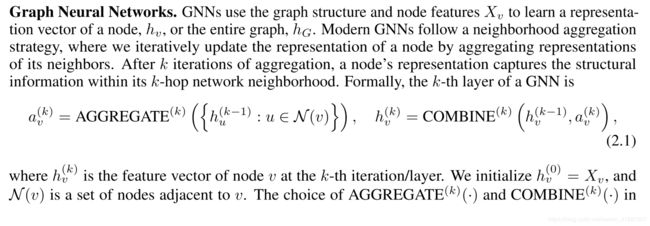
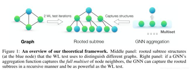
图1：我们的理论框架概述。 中间面板：有根的子树结构

（在蓝色节点处）WL测试用于区分不同的图形。 右图：如果GNN的聚合函数捕获节点邻居的完整多集节点，则GNN可以以递归方式捕获根节化子树，并且与WL测试一样强大。

GNN是至关重要的。 已经提出了许多用于AGGREGATE的架构。 在GraphSAGE的汇集变体中（Hamilton等，2017a），AGGREGATE已被公式化为

READOUT can be a simple permutation invariant function such as summation or a more sophisticated graph-level pooling function (Ying et al., 2018; Zhang et al., 2018).

Weisfeiler-Lehman test. The graph isomorphism problem asks whether two graphs are topologically identical. This is a challenging problem: no polynomial-time algorithm is known for it yet (Garey, 1979; Garey & Johnson, 2002; Babai, 2016). Apart from some corner cases (Cai et al., 1992), the Weisfeiler-Lehman (WL) test of graph isomorphism (Weisfeiler & Lehman, 1968) is an effective and computationally efficient test that distinguishes a broad class of graphs (Babai & Kucera, 1979). Its 1-dimensional form, “naïve vertex refinement”, is analogous to neighbor aggregation in GNNs. The WL test iteratively (1) aggregates the labels of nodes and their neighborhoods, and (2) hashes the aggregated labels into unique new labels. The algorithm decides that two graphs are non-isomorphic if at some iteration the labels of the nodes between the two graphs differ.

Based on the WL test, Shervashidze et al. (2011) proposed the WL subtree kernel that measures the similarity between graphs. The kernel uses the counts of node labels at different iterations of the WL test as the feature vector of a graph. Intuitively, a node’s label at the k-th iteration of WL test represents a subtree structure of height k rooted at the node (Figure 1). Thus, the graph features considered by the WL subtree kernel are essentially counts of different rooted subtrees in the graph.
READOUT可以是简单的置换不变函数，例如求和或更复杂的图级集合函数（Ying等，2018; Zhang等，2018）。

Weisfeiler-Lehman测试。图同构问题询问两个图是否在拓扑上相同。这是一个具有挑战性的问题：尚未知道多项式时间算法（Garey，1979; Garey＆Johnson，2002; Babai，2016）。除了一些极端情况（Cai et al。，1992），图同构的Weisfeiler-Lehman（WL）检验（Weisfeiler＆Lehman，1968）是一种有效且计算效率高的测试，可以区分广泛的图形（Babai和Kucera） ，1979）。它的一维形式“天真的顶点细化”类似于GNN中的邻居聚合。迭代地进行WL测试（1）聚合节点及其邻域的标签，以及（2）将聚合的标签散列为唯一的新标签。如果在某个迭代中两个图之间的节点的标签不同，则算法确定两个图是非同构的。

基于WL测试，Shervashidze等。 （2011）提出了测量图之间相似性的WL子树内核。内核使用WL测试的不同迭代中的节点标签的计数作为图的特征向量。直观地，WL测试的第k次迭代中的节点标签表示以节点为根的高度k的子树结构（图1）。因此，WL子树内核考虑的图形特征基本上是图中不同的有根子树的计数。

3 THEORETICAL FRAMEWORK: OVERVIEW

We start with an overview of our framework for analyzing the expressive power of GNNs. Figure 1 illustrates our idea. A GNN recursively updates each node’s feature vector to capture the network structure and features of other nodes around it, i.e., its rooted subtree structures (Figure 1). Throughout the paper, we assume node input features are from a countable universe. For finite graphs, node feature vectors at deeper layers of any fixed model are also from a countable universe. For notational simplicity, we can assign each feature vector a unique label in fa; b; c : : :g. Then, feature vectors of a set of neighboring nodes form a multiset (Figure 1): the same element can appear multiple times since different nodes can have identical feature vectors.
我们首先概述了分析GNN表达能力的框架。 图1说明了我们的想法。 GNN以递归方式更新每个节点的特征向量，以捕获网络结构和其周围其他节点的特征，即其根节子树结构（图1）。 在整篇论文中，我们假设节点输入特征来自可数的宇宙。 对于有限图，任何固定模型的较深层的节点特征向量也来自可数的宇宙。 为了简化符号，我们可以在fa中为每个特征向量分配一个唯一的标签;b; c ::: g。 然后，一组相邻节点的特征向量形成多集（图1）：相同的元素可以出现多次，因为不同的节点可以具有相同的特征向量。

To study the representational power of a GNN, we analyze when a GNN maps two nodes to the same location in the embedding space. Intuitively, a maximally powerful GNN maps two nodes to the same location only if they have identical subtree structures with identical features on the corresponding nodes. Since subtree structures are defined recursively via node neighborhoods (Figure 1), we can reduce our analysis to the question whether a GNN maps two neighborhoods (i.e., two multisets) to the same embedding or representation. A maximally powerful GNN would never map two different neighborhoods, i.e., multisets of feature vectors, to the same representation. This means its aggregation scheme must be injective. Thus, we abstract a GNN’s aggregation scheme as a class of functions over multisets that their neural networks can represent, and analyze whether they are able to represent injective multiset functions.

Next, we use this reasoning to develop a maximally powerful GNN. In Section 5, we study popular GNN variants and see that their aggregation schemes are inherently not injective and thus less powerful, but that they can capture other interesting properties of graphs.
为了研究GNN的表示能力，我们分析了GNN何时将两个节点映射到嵌入空间中的相同位置。直观地说，最强大的GNN只有在相应节点上具有相同特征的相同子树结构时才将两个节点映射到同一位置。由于子树结构是通过节点邻域递归定义的（图1），我们可以将我们的分析简化为GNN是否将两个邻域（即两个多集）映射到相同的嵌入或表示的问题。最强大的GNN永远不会将两个不同的邻域（即，多个特征向量）映射到相同的表示。这意味着它的聚合方案必须是单射的。因此，我们将GNN的聚合方案抽象为其神经网络可以表示的多个集合上的一类函数，并分析它们是否能够表示内射多集函数。

接下来，我们使用这种推理来开发一个最强大的GNN。在第5节中，我们研究了流行的GNN变体，并发现它们的聚合方案本质上不是单射的，因此功能较弱，但它们可以捕获图形的其他有趣属性。

4 BUILDING POWERFUL GRAPH NEURAL NETWORKS

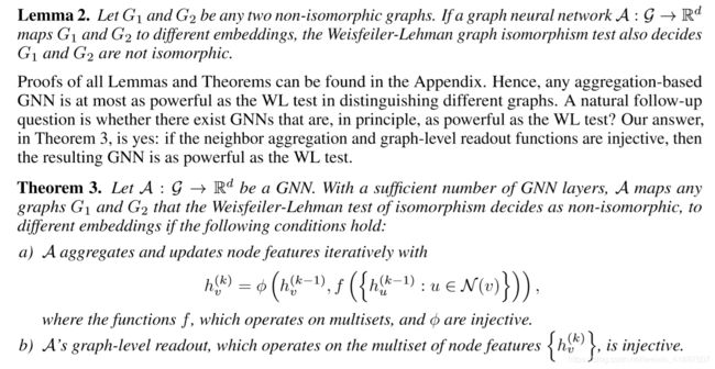
First, we characterize the maximum representational capacity of a general class of GNN-based models. Ideally, a maximally powerful GNN could distinguish different graph structures by mapping them to different representations in the embedding space. This ability to map any two different graphs to different embeddings, however, implies solving the challenging graph isomorphism problem. That is, we want isomorphic graphs to be mapped to the same representation and non-isomorphic ones to different representations. In our analysis, we characterize the representational capacity of GNNs via a slightly weaker criterion: a powerful heuristic called Weisfeiler-Lehman (WL) graph isomorphism test, that is known to work well in general, with a few exceptions, e.g., regular graphs (Cai et al., 1992; Douglas, 2011; Evdokimov & Ponomarenko, 1999).

首先，我们描述了一类基于GNN的模型的最大表示能力。 理想情况下，最强大的GNN可以通过将它们映射到嵌入空间中的不同表示来区分不同的图形结构。 然而，这种将任意两个不同图形映射到不同嵌入的能力意味着解决具有挑战性的图形同构问题。 也就是说，我们希望将同构图映射到相同的表示，将非同构图映射到不同的表示。 在我们的分析中，我们通过稍微弱一点的标准来描述GNN的表征能力：一种强大的启发式方法，称为Weisfeiler-Lehman（WL）图同构测试，已知它在一般情况下运行良好，但有一些例外，例如常规图（ Cai等，1992; Douglas，2011; Evdokimov＆Ponomarenko，1999）。

We prove Theorem 3 in the appendix. For countable sets, injectiveness well characterizes whether a function preserves the distinctness of inputs. Uncountable sets, where node features are continuous, need some further considerations. In addition, it would be interesting to characterize how close together the learned features lie in a function’s image. We leave these questions for future work, and focus on the case where input node features are from a countable set (that can be a subset of an uncountable set such as Rn).
我们在附录中证明了定理3。 对于可数集，内射性很好地表征函数是否保持输入的清晰度。 节点特征连续的不可计数集需要进一步考虑。 此外，描述学习特征在函数图像中的接近程度是很有趣的。 我们将这些问题留待将来工作，并关注输入节点特征来自可数集（可以是诸如Rn的不可数集的子集）的情况。

Here, it is also worth discussing an important benefit of GNNs beyond distinguishing different graphs, that is, capturing similarity of graph structures. Note that node feature vectors in the WL test are essentially one-hot encodings and thus cannot capture the similarity between subtrees. In contrast, a GNN satisfying the criteria in Theorem 3 generalizes the WL test by learning to embed the subtrees to low-dimensional space. This enables GNNs to not only discriminate different structures, but also to learn to map similar graph structures to similar embeddings and capture dependencies between graph structures. Capturing structural similarity of the node labels is shown to be helpful for generalization particularly when the co-occurrence of subtrees is sparse across different graphs or there are noisy edges and node features (Yanardag & Vishwanathan, 2015).
在这里，除了区分不同的图之外，还有必要讨论GNN的一个重要好处，即捕获图结构的相似性。 注意，WL测试中的节点特征向量基本上是单热编码，因此不能捕获子树之间的相似性。 相反，满足定理3中的标准的GNN通过学习将子树嵌入到低维空间来概括WL测试。 这使得GNN不仅可以区分不同的结构，还可以学习将类似的图形结构映射到类似的嵌入并捕获图形结构之间的依赖关系。 捕获节点标签的结构相似性被证明有助于推广，特别是当子树的共同出现在不同的图形上或者存在噪声边缘和节点特征时（Yanardag＆Vishwanathan，2015）。

4.1 GRAPH ISOMORPHISM NETWORK (GIN)

Having developed conditions for a maximally powerful GNN, we next develop a simple architecture, Graph Isomorphism Network (GIN), that provably satisfies the conditions in Theorem 3. This model generalizes the WL test and hence achieves maximum discriminative power among GNNs.

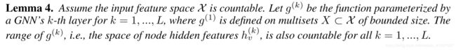
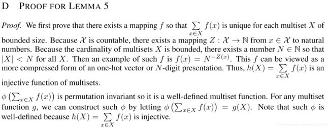
To model injective multiset functions for the neighbor aggregation, we develop a theory of “deep multisets”, i.e., parameterizing universal multiset functions with neural networks. Our next lemma states that sum aggregators can represent injective, in fact, universal functions over multisets.
为最强大的GNN开发了条件后，我们接下来开发了一个简单的架构，即图形同构网络（GIN），它可以证明满足定理3中的条件。该模型推广了WL测试，因此在GNN之间实现了最大的判别力。

为了模拟邻居聚合的内射多集函数，我们开发了一个“深多重集”理论，即用神经网络参数化通用多集函数。 我们的下一个引理表明，求和聚合器可以表示多重集合的内射，事实上，通用函数。

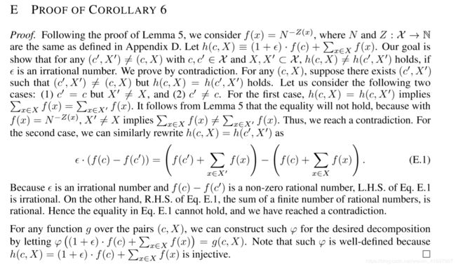
We prove Lemma 5 in the appendix. The proof extends the setting in (Zaheer et al., 2017) from sets to multisets. An important distinction between deep multisets and sets is that certain popular injective set functions, such as the mean aggregator, are not injective multiset functions. With the mechanism for modeling universal multiset functions in Lemma 5 as a building block, we can conceive aggregation schemes that can represent universal functions over a node and the multiset of its neighbors, and thus will satisfy the injectiveness condition (a) in Theorem 3. Our next corollary provides a simple and concrete formulation among many such aggregation schemes.
我们在附录中证明了引理5。 该证明将（Zaheer等，2017）的设置从集合扩展到多集合。 深度多集和集合之间的一个重要区别是某些流行的内射集函数，例如均值聚合器，不是内射多集函数。 利用引理5中的通用多集函数建模机制作为构建块，我们可以设想可以表示节点上的泛函和其邻域的多集的聚合方案，从而满足定理3中的内射条件（a）。 我们的下一个推论在许多这样的聚合方案中提供了简单而具体的公式。

Generally, there may exist many other powerful GNNs. GIN is one such example among many maximally powerful GNNs, while being simple.
通常，可能存在许多其他强大的GNN。 GIN是许多最强大的GNN中的一个这样的例子，虽然很简单。

4.2 GRAPH-LEVEL READOUT OF GIN

Node embeddings learned by GIN can be directly used for tasks like node classification and link prediction. For graph classification tasks we propose the following “readout” function that, given embeddings of individual nodes, produces the embedding of the entire graph.

An important aspect of the graph-level readout is that node representations, corresponding to subtree structures, get more refined and global as the number of iterations increases. A sufficient number of iterations is key to achieving good discriminative power. Yet, features from earlier iterations may sometimes generalize better. To consider all structural information, we use information from all depths/iterations of the model. We achieve this by an architecture similar to Jumping Knowledge
GIN学习的节点嵌入可以直接用于节点分类和链接预测等任务。 对于图分类任务，我们提出以下“读出”函数，给定单个节点的嵌入，产生整个图的嵌入。

图级读出的一个重要方面是，随着迭代次数的增加，对应于子树结构的节点表示变得更加精细和全局。 足够数量的迭代是实现良好判别力的关键。 然而，早期迭代的特征有时可能更好地概括。 为了考虑所有结构信息，我们使用来自模型的所有深度/迭代的信息。 我们通过类似于Jumping Knowledge的架构来实现这一目标

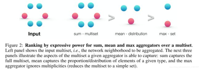
图2：通过多重集合中的sum，mean和max聚合器的表达能力排名。 左侧面板显示输入多集，即要聚合的网络邻域。 接下来的三个面板说明了给定聚合器能够捕获的多重集的各个方面：sum捕获完整的multiset，mean捕获给定类型的元素的比例/分布，max aggregator忽略多重性（将multiset简化为简单 组）。

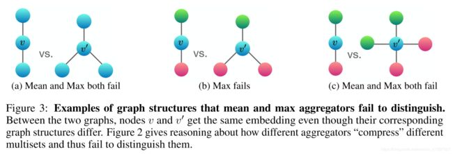
图3：平均值和最大聚合器无法区分的图结构示例。 在两个图之间，节点v和v0得到相同的嵌入，即使它们相应的图形结构不同。 图2给出了关于不同聚合器如何“压缩”不同多重集合并因此无法区分它们的推理。

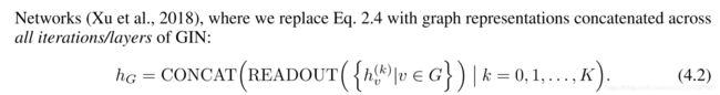
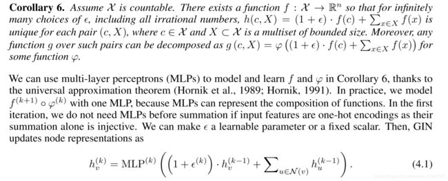
By Theorem 3 and Corollary 6, if GIN replaces READOUT in Eq. 4.2 with summing all node features from the same iterations (we do not need an extra MLP before summation for the same reason as in Eq. 4.1), it provably generalizes the WL test and the WL subtree kernel.
根据定理3和推论6，如果GIN取代了Eq中的READOUT。 4.2总结来自相同迭代的所有节点特征（在求和之前我们不需要额外的MLP，原因与方程4.1相同），它可以推广WL测试和WL子树内核。

5 LESS POWERFUL BUT STILL INTERESTING GNNS

Next, we study GNNs that do not satisfy the conditions in Theorem 3, including GCN (Kipf & Welling, 2017) and GraphSAGE (Hamilton et al., 2017a). We conduct ablation studies on two aspects of the aggregator in Eq. 4.1: (1) 1-layer perceptrons instead of MLPs and (2) mean or max-pooling instead of the sum. We will see that these GNN variants get confused by surprisingly simple graphs and are less powerful than the WL test. Nonetheless, models with mean aggregators like GCN perform well for node classification tasks. To better understand this, we precisely characterize what different GNN variants can and cannot capture about a graph and discuss the implications for learning with graphs.
接下来，我们研究不满足定理3中条件的GNN，包括GCN（Kipf＆Welling，2017）和GraphSAGE（Hamilton等，2017a）。 我们对方程式中聚合器的两个方面进行消融研究。 4.1：（1）1层感知器代替MLP和（2）平均或最大池而不是总和。 我们将看到这些GNN变体被令人惊讶的简单图形弄糊涂，并且不如WL测试强大。 尽管如此，具有平均聚合器（如GCN）的模型在节点分类任务中表现良好。 为了更好地理解这一点，我们精确地描述了不同的GNN变体能够和不能捕获关于图形的内容并讨论用图形学习的含义。

5.1 1-LAYER PERCEPTRONS ARE NOT SUFFICIENT

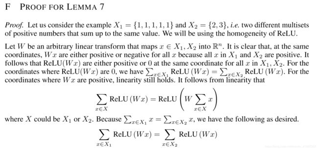
The function f in Lemma 5 helps map distinct multisets to unique embeddings. It can be param-eterized by an MLP by the universal approximation theorem (Hornik, 1991). Nonetheless, many existing GNNs instead use a 1-layer perceptron W (Duvenaud et al., 2015; Kipf & Welling, 2017; Zhang et al., 2018), a linear mapping followed by a non-linear activation function such as a ReLU. Such 1-layer mappings are examples of Generalized Linear Models (Nelder & Wedderburn, 1972). Therefore, we are interested in understanding whether 1-layer perceptrons are enough for graph learning. Lemma 7 suggests that there are indeed network neighborhoods (multisets) that models with 1-layer perceptrons can never distinguish.
引理5中的函数f有助于将不同的多集合映射到唯一的嵌入。 它可以通过MLP通过通用逼近定理进行参数化（Hornik，1991）。 尽管如此，许多现有的GNN代替使用1层感知器W（Duvenaud等，2015; Kipf＆Welling，2017; Zhang等，2018），线性映射后跟非线性激活函数，如ReLU。 这种1层映射是广义线性模型的例子（Nelder＆Wedderburn，1972）。 因此，我们有兴趣了解1层感知器是否足以进行图形学习。 引理7表明确实存在网络邻域（多重集合），具有1层感知器的模型永远无法区分。

The main idea of the proof for Lemma 7 is that 1-layer perceptrons can behave much like linear mappings, so the GNN layers degenerate into simply summing over neighborhood features. Our proof builds on the fact that the bias term is lacking in the linear mapping. With the bias term and sufficiently large output dimensionality, 1-layer perceptrons might be able to distinguish different multisets. Nonetheless, unlike models using MLPs, the 1-layer perceptron (even with the bias term) is not a universal approximator of multiset functions. Consequently, even if GNNs with 1-layer perceptrons can embed different graphs to different locations to some degree, such embeddings may not adequately capture structural similarity, and can be difficult for simple classifiers, e.g., linear classifiers, to fit. In Section 7, we will empirically see that GNNs with 1-layer perceptrons, when applied to graph classification, sometimes severely underfit training data and often perform worse than GNNs with MLPs in terms of test accuracy.
引理7证明的主要思想是1层感知器的行为很像线性映射，因此GNN层退化为简单地对邻域特征求和。我们的证据建立在线性映射中缺少偏差项的事实上。利用偏差项和足够大的输出维数，1层感知器可能能够区分不同的多重集。尽管如此，与使用MLP的模型不同，1层感知器（即使具有偏置项）也不是多集函数的通用逼近器。因此，即使具有1层感知器的GNN可以在一定程度上将不同的图形嵌入到不同的位置，这种嵌入也可能不能充分地捕获结构相似性，并且对于简单的分类器（例如，线性分类器）来说可能难以拟合。在第7节中，我们将凭经验看到具有1层感知器的GNN，当应用于图分类时，有时严重欠训练数据并且在测试准确性方面通常比具有MLP的GNN更差。

5.2 STRUCTURES THAT CONFUSE MEAN AND MAX-POOLING

What happens if we replace the sum in h (X) = x2X f(x) 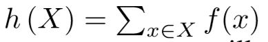with mean or max-pooling as in GCN and GraphSAGE? Mean and max-pooling aggregators are still well-defined multiset functions because they are permutation invariant. But, they are not injective. Figure 2 ranks the three aggregators by their representational power, and Figure 3 illustrates pairs of structures that the mean and max-pooling aggregators fail to distinguish. Here, node colors denote different node features, and we assume the GNNs aggregate neighbors first before combining them with the central node labeled as v and v0.

In Figure 3a, every node has the same feature a and f(a) is the same across all nodes (for any function f). When performing neighborhood aggregation, the mean or maximum over f(a) remains f(a) and, by induction, we always obtain the same node representation everywhere. Thus, in this case mean and max-pooling aggregators fail to capture any structural information. In contrast, the sum aggregator distinguishes the structures because 2 f(a) and 3 f(a) give different values. The same argument can be applied to any unlabeled graph. If node degrees instead of a constant value is used as node input features, in principle, mean can recover sum, but max-pooling cannot.
GCN和GraphSAGE？均值和最大池聚合器仍然是明确定义的多集函数，因为它们是排列不变的。但是，它们不是单射的。图2按其代表性功率对三个聚合器进行排名，图3显示了均值和最大池聚合器无法区分的结构对。这里，节点颜色表示不同的节点特征，并且我们假设GNN在将它们与标记为v和v0的中心节点组合之前首先聚合邻居。

在图3a中，每个节点具有相同的特征a，并且f（a）在所有节点上是相同的（对于任何函数f）。当执行邻域聚合时，f（a）上的均值或最大值仍为f（a），并且通过归纳，我们总是在任何地方获得相同的节点表示。因此，在这种情况下，均值和最大池聚合器无法捕获任何结构信息。相反，和聚合器区分结构，因为2 f（a）和3 f（a）给出不同的值。相同的参数可以应用于任何未标记的图形。如果节点度而不是常量值用作节点输入要素，原则上，均值可以恢复总和，但最大池不能。

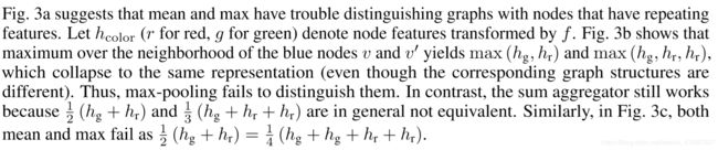
The mean aggregator may perform well if, for the task, the statistical and distributional information in the graph is more important than the exact structure. Moreover, when node features are diverse and rarely repeat, the mean aggregator is as powerful as the sum aggregator. This may explain why, despite the limitations identified in Section 5.2, GNNs with mean aggregators are effective for node classification tasks, such as classifying article subjects and community detection, where node features are rich and the distribution of the neighborhood features provides a strong signal for the task.
如果对于任务，图中的统计和分布信息比精确结构更重要，则平均聚合器可以表现良好。 此外，当节点特征多样且很少重复时，平均聚合器与总和聚合器一样强大。 这可以解释为什么，尽管第5.2节中确定了限制，具有均值聚合器的GNN对于节点分类任务是有效的，例如对文章主题和社区检测进行分类，其中节点特征丰富并且邻域特征的分布提供了强烈的信号。 任务。

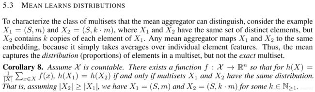
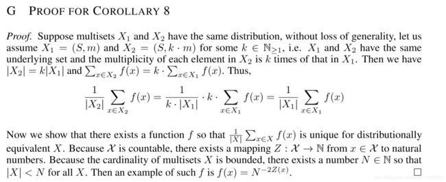
5.4 MAX-POOLING LEARNS SETS WITH DISTINCT ELEMENTS

The examples in Figure 3 illustrate that max-pooling considers multiple nodes with the same feature as only one node (i.e., treats a multiset as a set). Max-pooling captures neither the exact structure nor the distribution. However, it may be suitable for tasks where it is important to identify representative elements or the “skeleton”, rather than to distinguish the exact structure or distribution. Qi et al. (2017) empirically show that the max-pooling aggregator learns to identify the skeleton of a 3D point cloud and that it is robust to noise and outliers. For completeness, the next corollary shows that the max-pooling aggregator captures the underlying set of a multiset.
图3中的示例说明max-pooling认为具有与仅一个节点相同的特征的多个节点（即，将多个集合视为一组）。 最大池不捕获确切的结构和分布。 但是，它可能适用于识别代表性元素或“骨架”很重要的任务，而不是区分确切的结构或分布。 齐等人。 （2017）凭经验表明，最大池聚合器学习识别3D点云的骨架，并且它对噪声和异常值具有鲁棒性。 为了完整起见，下一个推论显示max-pooling聚合器捕获多集的基础集。

5.5 REMARKS ON OTHER AGGREGATORS

There are other non-standard neighbor aggregation schemes that we do not cover, e.g., weighted average via attention (Velickovic et al., 2018) and LSTM pooling (Hamilton et al., 2017a; Murphy et al., 2018). We emphasize that our theoretical framework is general enough to characterize the representaional power of any aggregation-based GNNs. In the future, it would be interesting to apply our framework to analyze and understand other aggregation schemes.
我们没有涉及其他非标准邻居聚合方案，例如，通过注意加权平均（Velickovic等，2018）和LSTM汇集（Hamilton等，2017a; Murphy等，2018）。 我们强调，我们的理论框架足以表征任何基于聚合的GNN的代表性能力。 将来，应用我们的框架来分析和理解其他聚合方案会很有趣。

6 OTHER RELATED WORK

Despite the empirical success of GNNs, there has been relatively little work that mathematically studies their properties. An exception to this is the work of Scarselli et al. (2009a) who shows that the perhaps earliest GNN model (Scarselli et al., 2009b) can approximate measurable functions in probability. Lei et al. (2017) show that their proposed architecture lies in the RKHS of graph kernels, but do not study explicitly which graphs it can distinguish. Each of these works focuses on a specific architecture and do not easily generalize to multple architectures. In contrast, our results above provide a general framework for analyzing and characterizing the expressive power of a broad class of GNNs. Recently, many GNN-based architectures have been proposed, including sum aggregation and MLP encoding (Battaglia et al., 2016; Scarselli et al., 2009b; Duvenaud et al., 2015), and most without theoretical derivation. In contrast to many prior GNN architectures, our Graph Isomorphism Network (GIN) is theoretically motivated, simple yet powerful.
尽管GNN取得了经验上的成功，但在数学上研究其性质的工作相对较少。一个例外是Scarselli等人的工作。 （2009a）谁表明，也许最早的GNN模型（Scarselli et al。，2009b）可以在概率上近似可测量的函数。雷等人。 （2017）表明他们提出的架构位于图形核的RKHS中，但没有明确地研究它可以区分哪些图。这些工作中的每一项都侧重于特定的体系结构，并且不容易推广到多种体系结构。相比之下，我们的结果提供了一个分析和表征广泛类GNN的表达能力的一般框架。最近，已经提出了许多基于GNN的体系结构，包括总和聚合和MLP编码（Battaglia等人，2016; Scarselli等人，2009b; Duvenaud等人，2015），并且大多数没有理论推导。与许多现有的GNN架构相比，我们的图形同构网络（GIN）在理论上是动机的，简单但功能强大。

7 EXPERIMENTS

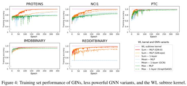
We evaluate and compare the training and test performance of GIN and less powerful GNN variants.1 Training set performance allows us to compare different GNN models based on their representational power and test set performance quantifies generalization ability.

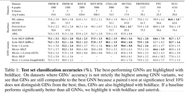
Datasets. We use 9 graph classification benchmarks: 4 bioinformatics datasets (MUTAG, PTC, NCI1, PROTEINS) and 5 social network datasets (COLLAB, IMDB-BINARY, IMDB-MULTI, REDDIT-BINARY and REDDIT-MULTI5K) (Yanardag & Vishwanathan, 2015). Importantly, our goal here is not to allow the models to rely on the input node features but mainly learn from the network structure. Thus, in the bioinformatic graphs, the nodes have categorical input features but in the social networks, they have no features. For social networks we create node features as follows: for the REDDIT datasets, we set all node feature vectors to be the same (thus, features here are uninformative); for the other social graphs, we use one-hot encodings of node degrees. Dataset statistics are summarized in Table 1, and more details of the data can be found in Appendix I.

Models and configurations. We evaluate GINs (Eqs. 4.1 and 4.2) and the less powerful GNN variants. Under the GIN framework, we consider two variants: (1) a GIN that learns in Eq. 4.1 by gradient descent, which we call GIN- , and (2) a simpler (slightly less powerful)2 GIN, where

in Eq. 4.1 is fixed to 0, which we call GIN-0. As we will see, GIN-0 shows strong empirical performance: not only does GIN-0 fit training data equally well as GIN- , it also demonstrates good generalization, slightly but consistently outperforming GIN- in terms of test accuracy. For the less powerful GNN variants, we consider architectures that replace the sum in the GIN-0 aggregation with mean or max-pooling3, or replace MLPs with 1-layer perceptrons, i.e., a linear mapping followed by ReLU. In Figure 4 and Table 1, a model is named by the aggregator/perceptron it uses. Here mean–1-layer and max–1-layer correspond to GCN and GraphSAGE, respectively, up to minor architecture modifications. We apply the same graph-level readout (READOUT in Eq. 4.2) for GINs and all the GNN variants, specifically, sum readout on bioinformatics datasets and mean readout on social datasets due to better test performance.
我们评估和比较GIN的训练和测试性能以及不太强大的GNN变体.1训练集性能允许我们基于它们的表征能力和测试集性能量化泛化能力来比较不同的GNN模型。

数据集。我们使用9个图表分类基准：4个生物信息学数据集（MUTAG，PTC，NCI1，PROTEINS）和5个社交网络数据集（COLLAB，IMDB-BINARY，IMDB-MULTI，REDDIT-BINARY和REDDIT-MULTI5K）（Yanardag＆Vishwanathan，2015） 。重要的是，我们的目标不是让模型依赖输入节点功能，而主要是从网络结构中学习。因此，在生物信息图中，节点具有分类输入特征，但是在社交网络中，它们没有特征。对于社交网络，我们按如下方式创建节点特征：对于REDDIT数据集，我们将所有节点特征向量设置为相同（因此，此处的特征无法提供信息）;对于其他社交图，我们使用节点度的单热编码。数据集统计数据总结在表1中，有关数据的更多详细信息，请参见附录I.

型号和配置。我们评估GIN（方程4.1和4.2）和不太强大的GNN变体。在GIN框架下，我们考虑两种变体：（1）在方程式中学习的GIN。 4.1通过梯度下降，我们称之为GIN-，和（2）更简单（稍微不那么强大）的2 GIN，其中

在Eq。 4.1固定为0，我们称之为GIN-0。正如我们将要看到的，GIN-0显示出强大的经验性能：GIN-0不仅与GIN一样适合训练数据，而且在测试精度方面也表现出良好的概括性，略微但始终优于GIN。对于功能较弱的GNN变体，我们考虑使用mean或max-pooling3替换GIN-0聚合中的总和的架构，或者用1层感知器替换MLP，即线性映射后跟ReLU。在图4和表1中，模型由它使用的聚合器/感知器命名。这里，mean-1-layer和max-1-layer分别对应于GCN和GraphSAGE，直到较小的架构修改。我们对GIN和所有GNN变体应用相同的图形级读数（公式4.2中的READOUT），特别是生物信息学数据集的总和读数和社交数据集的平均读数，因为更好的测试性能。

Following (Yanardag & Vishwanathan, 2015; Niepert et al., 2016), we perform 10-fold cross-validation with LIB-SVM (Chang & Lin, 2011). We report the average and standard deviation of validation accuracies across the 10 folds within the cross-validation. For all configurations, 5 GNN layers (including the input layer) are applied, and all MLPs have 2 layers. Batch normalization (Ioffe & Szegedy, 2015) is applied on every hidden layer. We use the Adam optimizer (Kingma

&Ba, 2015) with initial learning rate 0:01 and decay the learning rate by 0:5 every 50 epochs. The hyper-parameters we tune for each dataset are: (1) the number of hidden units 2 f16; 32g for bioinformatics graphs and 64 for social graphs; (2) the batch size 2 f32; 128g; (3) the dropout ratio 2 f0; 0:5g after the dense layer (Srivastava et al., 2014); (4) the number of epochs, i.e., a single epoch with the best cross-validation accuracy averaged over the 10 folds was selected. Note that due to the small dataset sizes, an alternative setting, where hyper-parameter selection is done using a validation set, is extremely unstable, e.g., for MUTAG, the validation set only contains 18 data points. We also report the training accuracy of different GNNs, where all the hyper-parameters were fixed across the datasets: 5 GNN layers (including the input layer), hidden units of size 64, minibatch of size 128, and 0.5 dropout ratio. For comparison, the training accuracy of the WL subtree kernel is reported, where we set the number of iterations to 4, which is comparable to the 5 GNN layers.

Baselines. We compare the GNNs above with a number of state-of-the-art baselines for graph classification: (1) the WL subtree kernel (Shervashidze et al., 2011), where C-SVM (Chang & Lin, 2011) was used as a classifier; the hyper-parameters we tune are C of the SVM and the number of WL iterations 2 f1; 2; : : : ; 6g; (2) state-of-the-art deep learning architectures, i.e., Diffusion-convolutional neural networks (DCNN) (Atwood & Towsley, 2016), PATCHY-SAN (Niepert et al., 2016) and Deep Graph CNN (DGCNN) (Zhang et al., 2018); (3) Anonymous Walk Embeddings (AWL) (Ivanov & Burnaev, 2018). For the deep learning methods and AWL, we report the accuracies reported in the original papers.
接下来（Yanardag＆Vishwanathan，2015; Niepert等，2016），我们使用LIB-SVM进行了10次交叉验证（Chang＆Lin，2011）。我们在交叉验证中报告了10倍的验证准确度的平均值和标准差。对于所有配置，应用5个GNN层（包括输入层），并且所有MLP具有2个层。批量标准化（Ioffe＆Szegedy，2015）应用于每个隐藏层。我们使用Adam优化器（Kingma

＆Ba，2015）初始学习率为0:01，并且每50个时期将学习率降低0：5。我们针对每个数据集调整的超参数是：（1）隐藏单元的数量2 f16;生物信息学图表为32g，社交图表为64; （2）批量2 f32; 128克; （3）辍学率2 f0;密集层后0：5g（Srivastava等，2014）; （4）选择时期数，即具有在10倍上平均的最佳交叉验证精度的单个时期。请注意，由于数据集大小较小，使用验证集进行超参数选择的替代设置非常不稳定，例如，对于MUTAG，验证集仅包含18个数据点。我们还报告了不同GNN的训练准确性，其中所有超参数在数据集中是固定的：5个GNN层（包括输入层），64个隐藏单位，128个小批量和0.5个丢失率。为了比较，报告了WL子树内核的训练精度，其中我们将迭代次数设置为4，这与5个GNN层相当。

基线。我们将上面的GNN与图形分类的一些最先进的基线进行比较：（1）WL子树内核（Shervashidze等，2011），其中使用了C-SVM（Chang＆Lin，2011）作为分类器;我们调谐的超参数是SVM的C和WL迭代的数量2 f1; 2; ::: ;; 6克; （2）最先进的深度学习架构，即扩散 - 卷积神经网络（DCNN）（Atwood＆Towsley，2016），PATCHY-SAN（Niepert等，2016）和Deep Graph CNN（DGCNN） （Zhang et al。，2018）; （3）Anonymous Walk Embeddings（AWL）（Ivanov＆Burnaev，2018）。对于深度学习方法和AWL，我们报告了原始论文中报告的准确性。

7.1 RESULTS

Training set performance. We validate our theoretical analysis of the representational power of GNNs by comparing their training accuracies. Models with higher representational power should have higher training set accuracy. Figure 4 shows training curves of GINs and less powerful GNN variants with the same hyper-parameter settings. First, both the theoretically most powerful GNN, i.e. GIN- and GIN-0, are able to almost perfectly fit all the training sets. In our experiments, explicit learning of in GIN- yields no gain in fitting training data compared to fixing to 0 as in GIN-0. In comparison, the GNN variants using mean/max pooling or 1-layer perceptrons severely underfit on many datasets. In particular, the training accuracy patterns align with our ranking by the models’ representational power: GNN variants with MLPs tend to have higher training accuracies than those with 1-layer perceptrons, and GNNs with sum aggregators tend to fit the training sets better than those with mean and max-pooling aggregators.
训练集表现。我们通过比较它们的训练精度来验证我们对GNN表征能力的理论分析。具有较高代表能力的模型应具有较高的训练集精度。图4显示了具有相同超参数设置的GIN和功能较弱的GNN变体的训练曲线。首先，理论上最强大的GNN，即GIN-和GIN-0，几乎完全适合所有训练集。在我们的实验中，与GIN-0中固定为0相比，GIN中的显式学习在拟合训练数据方面没有收益。相比之下，使用均值/最大池或1层感知器的GNN变体在许多数据集上严重不足。特别是，训练准确性模式与我们的模型表征能力排名一致：具有MLP的GNN变体往往比具有1层感知器的GNN变体具有更高的训练精度，并且具有总和聚合器的GNN倾向于比那些更好地适应训练集。使用均值和最大池聚合器。

On our datasets, training accuracies of the GNNs never exceed those of the WL subtree kernel. This is expected because GNNs generally have lower discriminative power than the WL test. For example, on IMDBBINARY, none of the models can perfectly fit the training set, and the GNNs achieve at most the same training accuracy as the WL kernel. This pattern aligns with our result that the WL test provides an upper bound for the representational capacity of the aggregation-based GNNs. However, the WL kernel is not able to learn how to combine node features, which might be quite informative for a given prediction task as we will see next.

Test set performance. Next, we compare test accuracies. Although our theoretical results do not directly speak about the generalization ability of GNNs, it is reasonable to expect that GNNs with strong expressive power can accurately capture graph structures of interest and thus generalize well. Table 1 compares test accuracies of GINs (Sum–MLP), other GNN variants, as well as the state-of-the-art baselines.

First, GINs, especially GIN-0, outperform (or achieve comparable performance as) the less powerful GNN variants on all the 9 datasets, achieving state-of-the-art performance. GINs shine on the social network datasets, which contain a relatively large number of training graphs. For the Reddit datasets, all nodes share the same scalar as node feature. Here, GINs and sum-aggregation GNNs accurately capture the graph structure and significantly outperform other models. Mean-aggregation GNNs, however, fail to capture any structures of the unlabeled graphs (as predicted in Section 5.2) and do not perform better than random guessing. Even if node degrees are provided as input features, mean-based GNNs perform much worse than sum-based GNNs (the accuracy of the GNN with mean– MLP aggregation is 71.2 4.6% on REDDIT-BINARY and 41.3 2.1% on REDDIT-MULTI5K). Comparing GINs (GIN-0 and GIN- ), we observe that GIN-0 slightly but consistently outperforms GIN- . Since both models fit training data equally well, the better generalization of GIN-0 may be explained by its simplicity compared to GIN- .
在我们的数据集上，GNN的训练精度永远不会超过WL子树内核的训练精度。这是预期的，因为GNN通常具有比WL测试更低的辨别力。例如，在IMDBBINARY上，没有一个模型可以完美地适应训练集，并且GNN最多可以实现与WL内核相同的训练精度。这种模式与我们的结果一致，即WL测试为基于聚合的GNN的表示能力提供了上限。但是，WL内核无法学习如何组合节点功能，这对于给定的预测任务可能非常有用，我们将在下面看到。

测试集性能。接下来，我们比较测试精度。虽然我们的理论结果并没有直接谈到GNN的泛化能力，但可以合理地预期具有强表达能力的GNN可以准确地捕获感兴趣的图结构，从而得到很好的推广。表1比较了GIN（Sum-MLP），其他GNN变体以及最先进基线的测试准确度。

首先，GIN，特别是GIN-0，在所有9个数据集上的强弱GNN变体的表现优于（或达到相当的性能），实现了最先进的性能。 GIN在社交网络数据集上闪耀，其中包含相对大量的训练图。对于Reddit数据集，所有节点与节点功能共享相同的标量。在这里，GIN和总和聚合GNN准确地捕获图形结构，并且明显优于其他模型。然而，均值聚合GNN无法捕获未标记图的任何结构（如第5.2节中所预测的），并且不如随机猜测表现更好。即使提供节点度作为输入特征，基于均值的GNN也比基于总和的GNN表现得差得多（GND与MLP聚合的准确度在REDDIT-BINARY上为71.2 4.6％，在REDDIT-MULTI5K上为41.3 2.1％） 。比较GIN（GIN-0和GIN-），我们观察到GIN-0略微但始终优于GIN-。由于两种模型都能很好地拟合训练数据，因此GIN-0的更好的推广可以通过与GIN相比的简单性来解释。

8 CONCLUSION

In this paper, we developed theoretical foundations for reasoning about the expressive power of GNNs, and proved tight bounds on the representational capacity of popular GNN variants. We also designed a provably maximally powerful GNN under the neighborhood aggregation framework. An interesting direction for future work is to go beyond neighborhood aggregation (or message passing) in order to pursue possibly even more powerful architectures for learning with graphs. To complete the picture, it would also be interesting to understand and improve the generalization properties of GNNs as well as better understand their optimization landscape.
在本文中，我们为推理GNNs的表达能力提供了理论基础，并证明了对流行GNN变体的表征能力的严格限制。 我们还在邻域聚合框架下设计了一个可证明最强大的GNN。 未来工作的一个有趣方向是超越邻域聚合（或消息传递），以便寻求可能更强大的架构来学习图形。 为了完成图片，理解和改进GNN的泛化属性以及更好地理解它们的优化环境也将是有趣的。

ACKNOWLEDGMENTS

This research was supported by NSF CAREER award 1553284, a DARPA D3M award and DARPA DSO’s Lagrange program under grant FA86501827838. This research was also supported in part by NSF, ARO MURI, Boeing, Huawei, Stanford Data Science Initiative, and Chan Zuckerberg Biohub. Weihua Hu was supported by Funai Overseas Scholarship. We thank Prof. Ken-ichi Kawarabayashi and Prof. Masashi Sugiyama for supporting this research with computing resources and providing great advice. We thank Tomohiro Sonobe and Kento Nozawa for managing servers. We thank Rex Ying and William Hamilton for helpful feedback. We thank Simon S. Du, Yasuo Tabei, Chengtao Li, and Jingling Li for helpful discussions and positive comments.
这项研究得到了NSF CAREER奖1553284，DARPA D3M奖和DARPA DSO的Lagrange计划资助FA86501827838的支持。 NSF，ARO MURI，波音，华为，斯坦福数据科学计划和Chan Zuckerberg Biohub也部分支持了这项研究。 胡伟华获得船井海外奖学金。 我们感谢Ken-ichi Kawarabayashi教授和Masashi Sugiyama教授用计算资源支持这项研究并提供了很好的建议。 我们感谢Tomohiro Sonobe和Kento Nozawa管理服务器。 我们感谢Rex Ying和William Hamilton提供了有用的反馈。 我们感谢Simon S. Du，Yasuo Tabei，Chengtao Li和Jingling Li的有益讨论和积极评论。

REFERENCES

James Atwood and Don Towsley. Diffusion-convolutional neural networks. In Advances in Neural Information Processing Systems (NIPS), pp. 1993–2001, 2016.

László Babai. Graph isomorphism in quasipolynomial time. In Proceedings of the forty-eighth annual ACM symposium on Theory of Computing, pp. 684–697. ACM, 2016.

László Babai and Ludik Kucera. Canonical labelling of graphs in linear average time. In Foundations of Computer Science, 1979., 20th Annual Symposium on, pp. 39–46. IEEE, 1979.

Peter Battaglia, Razvan Pascanu, Matthew Lai, Danilo Jimenez Rezende, et al. Interaction networks for learning about objects, relations and physics. In Advances in Neural Information Processing Systems (NIPS), pp. 4502–4510, 2016.

Jin-Yi Cai, Martin Fürer, and Neil Immerman. An optimal lower bound on the number of variables for graph identification. Combinatorica, 12(4):389–410, 1992.

Chih-Chung Chang and Chih-Jen Lin. Libsvm: a library for support vector machines. ACM transactions on intelligent systems and technology (TIST), 2(3):27, 2011.

Michaël Defferrard, Xavier Bresson, and Pierre Vandergheynst. Convolutional neural networks on graphs with fast localized spectral filtering. In Advances in Neural Information Processing Systems (NIPS), pp. 3844–3852, 2016.

Brendan L Douglas. The weisfeiler-lehman method and graph isomorphism testing. arXiv preprint arXiv:1101.5211, 2011.

David K Duvenaud, Dougal Maclaurin, Jorge Iparraguirre, Rafael Bombarell, Timothy Hirzel, Alán Aspuru-Guzik, and Ryan P Adams. Convolutional networks on graphs for learning molecular fingerprints. pp. 2224–2232, 2015.

Sergei Evdokimov and Ilia Ponomarenko. Isomorphism of coloured graphs with slowly increasing multiplicity of jordan blocks. Combinatorica, 19(3):321–333, 1999.

Michael R Garey. A guide to the theory of np-completeness. Computers and intractability, 1979.

Michael R Garey and David S Johnson. Computers and intractability, volume 29. wh freeman New York, 2002.

Justin Gilmer, Samuel S Schoenholz, Patrick F Riley, Oriol Vinyals, and George E Dahl. Neural message passing for quantum chemistry. In International Conference on Machine Learning (ICML), pp. 1273–1272, 2017.

William L Hamilton, Rex Ying, and Jure Leskovec. Inductive representation learning on large graphs.

In Advances in Neural Information Processing Systems (NIPS), pp. 1025–1035, 2017a.

William L Hamilton, Rex Ying, and Jure Leskovec. Representation learning on graphs: Methods and applications. IEEE Data Engineering Bulletin, 40(3):52–74, 2017b.

Kurt Hornik. Approximation capabilities of multilayer feedforward networks. Neural networks, 4(2):

251–257, 1991.

Kurt Hornik, Maxwell Stinchcombe, and Halbert White. Multilayer feedforward networks are universal approximators. Neural networks, 2(5):359–366, 1989.

Sergey Ioffe and Christian Szegedy. Batch normalization: Accelerating deep network training by reducing internal covariate shift. In International Conference on Machine Learning (ICML), pp. 448–456, 2015.

Sergey Ivanov and Evgeny Burnaev. Anonymous walk embeddings. In International Conference on Machine Learning (ICML), pp. 2191–2200, 2018.

Steven Kearnes, Kevin McCloskey, Marc Berndl, Vijay Pande, and Patrick Riley. Molecular graph convolutions: moving beyond fingerprints. Journal of computer-aided molecular design, 30(8): 595–608, 2016.

Diederik P Kingma and Jimmy Ba. Adam: A method for stochastic optimization. In International Conference on Learning Representations (ICLR), 2015.

Thomas N Kipf and Max Welling. Semi-supervised classification with graph convolutional networks.

In International Conference on Learning Representations (ICLR), 2017.

Tao Lei, Wengong Jin, Regina Barzilay, and Tommi Jaakkola. Deriving neural architectures from sequence and graph kernels. pp. 2024–2033, 2017.

Yujia Li, Daniel Tarlow, Marc Brockschmidt, and Richard Zemel. Gated graph sequence neural networks. In International Conference on Learning Representations (ICLR), 2016.

Ryan L Murphy, Balasubramaniam Srinivasan, Vinayak Rao, and Bruno Ribeiro. Janossy pool-ing: Learning deep permutation-invariant functions for variable-size inputs. arXiv preprint arXiv:1811.01900, 2018.

J. A. Nelder and R. W. M. Wedderburn. Generalized linear models. Journal of the Royal Statistical Society, Series A, General, 135:370–384, 1972.

Mathias Niepert, Mohamed Ahmed, and Konstantin Kutzkov. Learning convolutional neural networks for graphs. In International Conference on Machine Learning (ICML), pp. 2014–2023, 2016.

Charles R Qi, Hao Su, Kaichun Mo, and Leonidas J Guibas. Pointnet: Deep learning on point sets for 3d classification and segmentation. Proc. Computer Vision and Pattern Recognition (CVPR), IEEE, 1(2):4, 2017.

Adam Santoro, David Raposo, David G Barrett, Mateusz Malinowski, Razvan Pascanu, Peter Battaglia, and Timothy Lillicrap. A simple neural network module for relational reasoning. In Advances in neural information processing systems, pp. 4967–4976, 2017.

Adam Santoro, Felix Hill, David Barrett, Ari Morcos, and Timothy Lillicrap. Measuring abstract reasoning in neural networks. In International Conference on Machine Learning, pp. 4477–4486, 2018.

Franco Scarselli, Marco Gori, Ah Chung Tsoi, Markus Hagenbuchner, and Gabriele Monfardini. Computational capabilities of graph neural networks. IEEE Transactions on Neural Networks, 20
(1):81–102, 2009a.

Franco Scarselli, Marco Gori, Ah Chung Tsoi, Markus Hagenbuchner, and Gabriele Monfardini. The graph neural network model. IEEE Transactions on Neural Networks, 20(1):61–80, 2009b.

Nino Shervashidze, Pascal Schweitzer, Erik Jan van Leeuwen, Kurt Mehlhorn, and Karsten M Borgwardt. Weisfeiler-lehman graph kernels. Journal of Machine Learning Research, 12(Sep): 2539–2561, 2011.

Nitish Srivastava, Geoffrey Hinton, Alex Krizhevsky, Ilya Sutskever, and Ruslan Salakhutdinov. Dropout: a simple way to prevent neural networks from overfitting. The Journal of Machine Learning Research, 15(1):1929–1958, 2014.

Petar Velickovic, Guillem Cucurull, Arantxa Casanova, Adriana Romero, Pietro Lio, and Yoshua Bengio. Graph attention networks. In International Conference on Learning Representations (ICLR), 2018.

Saurabh Verma and Zhi-Li Zhang. Graph capsule convolutional neural networks. arXiv preprint arXiv:1805.08090, 2018.

Boris Weisfeiler and AA Lehman. A reduction of a graph to a canonical form and an algebra arising during this reduction. Nauchno-Technicheskaya Informatsia, 2(9):12–16, 1968.

Keyulu Xu, Chengtao Li, Yonglong Tian, Tomohiro Sonobe, Ken-ichi Kawarabayashi, and Stefanie Jegelka. Representation learning on graphs with jumping knowledge networks. In International Conference on Machine Learning (ICML), pp. 5453–5462, 2018.

Pinar Yanardag and SVN Vishwanathan. Deep graph kernels. In Proceedings of the 21th ACM SIGKDD International Conference on Knowledge Discovery and Data Mining, pp. 1365–1374. ACM, 2015.

Rex Ying, Jiaxuan You, Christopher Morris, Xiang Ren, William L Hamilton, and Jure Leskovec. Hierarchical graph representation learning with differentiable pooling. In Advances in Neural Information Processing Systems (NIPS), 2018.

Manzil Zaheer, Satwik Kottur, Siamak Ravanbakhsh, Barnabas Poczos, Ruslan R Salakhutdinov, and Alexander J Smola. Deep sets. In Advances in Neural Information Processing Systems, pp. 3391–3401, 2017.

Muhan Zhang, Zhicheng Cui, Marion Neumann, and Yixin Chen. An end-to-end deep learning architecture for graph classification. In AAAI Conference on Artificial Intelligence, pp. 4438–4445, 2018.

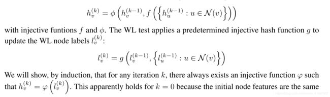
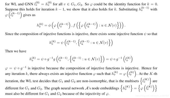
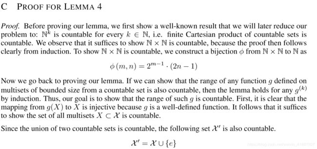
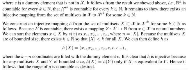
B PROOF FOR THEOREM 3

Proof. Let A be a graph neural network where the condition holds. Let G1, G2 be any graphs which the WL test decides as non-isomorphic at iteration K. Because the graph-level readout function is injective, i.e., it maps distinct multiset of node features into unique embeddings, it sufficies to show that A’s neighborhood aggregation process, with sufficient iterations, embeds G1 and G2 into different multisets of node features. Let us assume A updates node representations as
证明。 设A是条件成立的图神经网络。 设G1，G2为WL测试在迭代K时判定为非同构的任何图形。因为图形级读出函数是单射的，即它将不同的多节点节点特征映射到独特的嵌入，它足以证明A的邻域 聚合过程，通过足够的迭代，将G1和G2嵌入到不同的多节点节点特征中。 让我们假设A更新节点表示为

IDETAILS OF DATASETS

We give detailed descriptions of datasets used in our experiments. Further details can be found in (Yanardag & Vishwanathan, 2015).

Social networks datasets. IMDB-BINARY and IMDB-MULTI are movie collaboration datasets. Each graph corresponds to an ego-network for each actor/actress, where nodes correspond to ac-tors/actresses and an edge is drawn betwen two actors/actresses if they appear in the same movie. Each graph is derived from a pre-specified genre of movies, and the task is to classify the genre graph it is derived from. REDDIT-BINARY and REDDIT-MULTI5K are balanced datasets where each graph corresponds to an online discussion thread and nodes correspond to users. An edge was drawn between two nodes if at least one of them responded to another’s comment. The task is to classify each graph to a community or a subreddit it belongs to. COLLAB is a scientific collaboration dataset, derived from 3 public collaboration datasets, namely, High Energy Physics, Condensed Matter Physics and Astro Physics. Each graph corresponds to an ego-network of different researchers from each field. The task is to classify each graph to a field the corresponding researcher belongs to.

Bioinformatics datasets. MUTAG is a dataset of 188 mutagenic aromatic and heteroaromatic nitro compounds with 7 discrete labels. PROTEINS is a dataset where nodes are secondary structure elements (SSEs) and there is an edge between two nodes if they are neighbors in the amino-acid sequence or in 3D space. It has 3 discrete labels, representing helix, sheet or turn. PTC is a dataset of 344 chemical compounds that reports the carcinogenicity for male and female rats and it has 19 discrete labels. NCI1 is a dataset made publicly available by the National Cancer Institute (NCI) and is a subset of balanced datasets of chemical compounds screened for ability to suppress or inhibit the growth of a panel of human tumor cell lines, having 37 discrete labels.

IDATAILS OF DATASETS

我们详细描述了我们实验中使用的数据集。更多细节可以在（Yanardag＆Vishwanathan，2015）中找到。

社交网络数据集。 IMDB-BINARY和IMDB-MULTI是电影协作数据集。每个图对应于每个演员/女演员的自我网络，其中节点对应于演员/女演员，并且如果两个演员/女演员出现在同一电影中，则边缘被绘制。每个图表都是从预先指定的电影类型中派生出来的，任务是对其派生的类型图进行分类。 REDDIT-BINARY和REDDIT-MULTI5K是平衡数据集，其中每个图对应于在线讨论线程，节点对应于用户。如果两个节点中至少有一个响应另一个节点，则在两个节点之间绘制一条边。任务是将每个图表分类为它所属的社区或subreddit。 COLLAB是一个科学合作数据集，源自3个公共协作数据集，即高能物​​理，凝聚态物理和天文物理。每个图对应于来自每个领域的不同研究人员的自我网络。任务是将每个图分类到相应研究人员所属的字段。

生物信息学数据集。 MUTAG是188种诱变芳香族和杂芳族硝基化合物的数据集，具有7个离散标记。 PROTEINS是一个数据集，其中节点是二级结构元素（SSE），如果它们是氨基酸序列或3D空间中的邻居，则在两个节点之间存在边缘。它有3个离散标签，分别代表螺旋，片或转。 PTC是344种化合物的数据集，报告了雄性和雌性大鼠的致癌性，它有19个不连续的标记。 NCI1是由国家癌症研究所（NCI）公开提供的数据集，并且是筛选具有37个离散标记的抑制或抑制一组人肿瘤细胞系生长的能力的化学化合物的平衡数据集的子集。