机器学习(Machine Learning)基础

机器学习(Machine Learning)基础

概念及用途

	专门研究计算机怎样模拟或实现人类的学习行为，以获取新的知识或技能，重新组织已有的知识结构使之不断改善自身的性能。它是人工智能的核心，是使计算机具有智能的根本途径。步骤就是根据历史数据训练机器模型，再将新的问题输入这个模型从而预测未知的事件。
	我们的日常生活中，很多地方都有涉及到机器学习，比如无人驾驶、人脸识别、语音交互以及时下比较热门的推进系统。

机器学习的分类

基于学习方式的分类可以分为有监督学习、无监督学习以及强化学习
1、监督学习：
训练样本包含对应的标签，即带答案的数据，又可以分为分类问题和回归问题。
分类问题：样本标签属于离散型变量（类别型变量），比如判断垃圾邮件或者是肿瘤检测等等；
回归问题：样本标签属于连续性变量（可以任意取值的变量），比如预测房价，预测销售额等等。
1.1、分类问题：可以分为生成模型（概率模型）和判别模型（非概率模型）
1.1.1、判别式模型举例：判别一只羊的种类，从一堆羊中提取特征学习到一个决策边界，然后提取这只羊的特征来放到模型里面进行判断是山羊或者是绵羊；
1.1.2、生成式模型举例：根据山羊的特征学习出一个山羊的模型，再根据绵羊的特征学习出一个绵羊的模型，然后从这只羊中提取特征，放到两个模型中，比较哪个概率比较大。
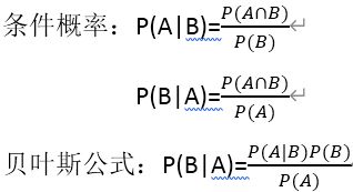
1.1.3、生成式模型用数据联合概率分布；
判别式模型使用条件概率直接预测；

2、无监督学习：
3、强化学习：

机器学习的流程

特征表示——选择模型——训练模型——模型评估

机器学习方法的三要素

1、模型：就是要学习的概率分布或者决策函数，所有可能的条件概率分布或者决策函数构成的集合，就是模型的假设空间。
2、策略：从假设空间中学习最优的模型的方法称为策略。
衡量模型好与不好需要一些指标，这时引入损失函数和风险函数来衡量，预测值和真实值通常是不相等的，我们用损失函数或者是代价函数来衡量预测错误的程度，记作

3、算法：算法是指学习模型时的具体计算方法，求解最优模型归结为一个最优化问题
统计学的算法等价于求解最优问题的算法，主要是求解、析解或者是数值解

机器学习算法的原理

1、线性回归或者是罗辑回归：
1.1、梯度下降算法：梯度下降是一个用来求函数最小值的算法。
1.2、梯度：在单变量的函数中，梯度其实就是函数的微分，代表着函数在某个给定点的切线斜率。在多变量函数中，梯度是对每个变量的偏微分组成的向量，梯度的方向就是这个向量的方向，它是函数在给定点的上升(下降)最快的方向。
1.3、梯度下降求极值点的原理：因为位于极值点的时候，梯度趋近于零，自变量的变化速度也会变小，当自变量的更新前后差值达到设定的阀值的时候，则停止迭代。
1.4、重复直至收敛：

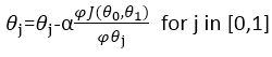
1.5、梯度下降法关键在于求出代价函数的导数：

梯度下降求函数极值点的方法：

import numpy as np
def f(x):
    return x**2-4*x+4
def h(x):
    return 2*x-4
a=16
step=0.1
count=0
deta_a=16
error_rate=1e-10
while deta_a>error_rate:
    a=a-step*h(a)
    deta_a=np.abs(deta_a-a)
    count+=1
print("梯度下降迭代第{}次".format(count,a,f(a)))
print("迭代次数%d"%count)
print("极值点为(%f,%f)"%(a,f(a)))

1.6、梯度下降的三种方法：批量梯度下降、随即梯度下降、小批量梯度下降。
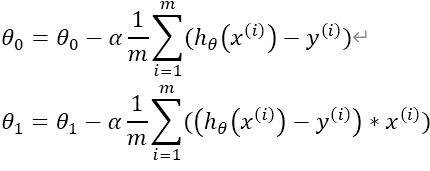
1.6.1、批量梯度下降（batch gradient decent）

(https://img-blog.csdnimg.cn/20191105201814447.bmp?x-oss-process=image/watermark,type_ZmFuZ3poZW5naGVpdGk,shadow_10,text_aHR0cHM6Ly9ibG9nLmNzZG4ubmV0L0FEd2Fpd2Fp,size_16,color_FFFFFF,t_70)

eta=0.1  #步长
n_iterations=1000  #迭代次数
m=100   #数据量
theta=np.random.randn(2,1)  #参数（两个）
for iteration in range(n_iterations):   #控制迭代次数
    gradients=2/m*X_b.T.dot(X_b.dot(theta)-y)  #求偏导
    theta=theta-eta*gradients   #更新theta值

theta_path_bgd=[]
def plot_gradient_descent(theta,eta,theta_path=None):    #定义
    m=len(X_b)
    plt.plot(X,y,"b.")   #画点
    n_iterations =1000
    for iteration in range(n_iterations):
        if iteration < 10:    #只显示前十条
            y_predict=X_new_b.dot(theta)
            style="b-"  #画实线
            plt.plot(X_new,y_predict,style)  #画回归线
        gradients=2/m*X_b.T.dot(X_b.dot(theta)-y)   #求偏导数
        theta=theta-eta*gradients  #更新theta值
        if theta_path is not None:
            theta_path.append(theta)
    plt.xlabel("$x_1$",fontsize=18)
    plt.axis([0,2,0,15])
    plt.title(r"$\eta={}$".format(eta),fontsize=16)
    

np.random.seed(42)
theta=np.random.randn(2,1)

plt.figure(figsize=(10,4))
plt.subplot(131);plot_gradient_descent(theta,eta=0.02)
plt.ylabel("$y$",rotation=0,fontsize=18)
plt.subplot(132);plot_gradient_descent(theta,eta=0.1,theta_path=theta_path_bgd)
plt.subplot(133);plot_gradient_descent(theta,eta=0.5)

save_fig("generated_data_plot")
plt.show()

https://img-blog.csdnimg.cn/20191105201952484.bmp?x-oss-process=image/watermark,type_ZmFuZ3poZW5naGVpdGk,shadow_10,text_aHR0cHM6Ly9ibG9nLmNzZG4ubmV0L0FEd2Fpd2Fp,size_16,color_FFFFFF,t_70
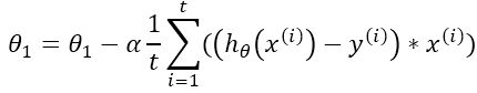
1.6.2、随即梯度下降（stochastic gradient decent）

```python
theta_path_sgd=[]
m=len(X_b)
np.random.seed(43)

n_epochs=50
theta=np.random.randn(2,1)  #随机初始化
for epoch in range(n_epochs):
    for i in range(m):
        if epoch==0 and i<20:
            y_predict=X_new_b.dot(theta)
            style="p-"
            plt.plot(X_new,y_predict,style)
        random_index=np.random.randint(m)
        xi=X_b[random_index:random_index+1]
        yi=y[random_index:random_index+1]
        gradients=2*xi.T.dot(xi.dot(theta)-yi)
        eta=0.1
        theta=theta-eta*gradients
        theta_path_sgd.append(theta)
plt.plot(X,y,"b.")
plt.xlabel("$x_1$",fontsize=18)
plt.ylabel("$y$",rotation=0,fontsize=18)
plt.axis([0,2,0,15])
save_fig("sgd_plot")
plt.show

https://img-blog.csdnimg.cn/20191105194448539.bmp?x-oss-process=image/watermark,type_ZmFuZ3poZW5naGVpdGk,shadow_10,text_aHR0cHM6Ly9ibG9nLmNzZG4ubmV0L0FEd2Fpd2Fp,size_16,color_FFFFFF,t_70

1.6.3、小批量梯度下降（mini-batch gradient decent）

theta_path_mgd=[]

n_iterations=50   #迭代次数
minibatch_size=20   #小批量的次数
np.random.seed(42)
theta=np.random.randn(2,1)
for epoch in range(n_iterations):
    shuffled_indices=np.random.permutation(m)
    X_b_shuffled=X_b[shuffled_indices]
    y_shuffled=y[shuffled_indices]
    for i in range(0,m,minibatch_size):
        xi=X_b_shuffled[i:i+minibatch_size]
        yi=y_shuffled[i:i+minibatch_size]
        gradients=2/minibatch_size*xi.T.dot(xi.dot(theta)-yi)
        eta=0.1
        theta=theta-eta*gradients
        theta_path_mgd.append(theta)
    
    
theta_path_bgd=np.array(theta_path_bgd)
theta_path_sgd=np.array(theta_path_sgd)
theta_path_mgd=np.array(theta_path_mgd)

plt.figure(figsize=(7,4))
plt.plot(theta_path_sgd[:,0],theta_path_sgd[:,1],"r-s",linewidth=1,label="Stochastic")
plt.plot(theta_path_mgd[:,0],theta_path_mgd[:,1],"g-+",linewidth=2,label="Mini-batch")
plt.plot(theta_path_bgd[:,0],theta_path_bgd[:,1],"b-o",linewidth=3,label="Batch")
plt.legend(loc="upper left",fontsize=16)
plt.xlabel(r"$\theta_0$",fontsize=20)
plt.ylabel(r"$\theta_1$",fontsize=20,rotation=0)
plt.axis([2.5,4.5,2.3,3.9])
save_fig("gradient_descent_paths_plot")
plt.show()

https://img-blog.csdnimg.cn/2019110519450018.bmp?x-oss-process=image/watermark,type_ZmFuZ3poZW5naGVpdGk,shadow_10,text_aHR0cHM6Ly9ibG9nLmNzZG4ubmV0L0FEd2Fpd2Fp,size_16,color_FFFFFF,t_70
2、决策树：
3、随即森林：
4、支持向量机：
5、朴素贝叶斯：
6、K近邻算法：
7、K均值算法：
8、Adaboost：
9、神经网络：
10、马尔科夫：