Faster-RCNN的Keras实现
Faster-RCNN的流程图
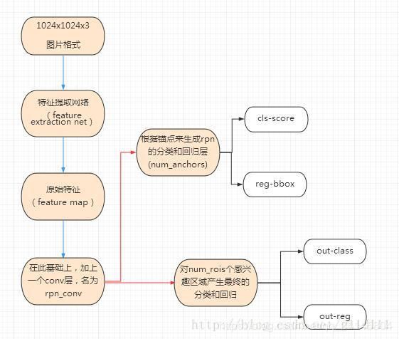
以下将根据流程图来简单介绍各个模块的实现。
数据预处理
我们采用物体检测最常用的数据集PASCAL VOC,包括VOC2007和VOC2012。将三个压缩包该数据集的目录结构是这样的:
VOCdevkit
VOC2007
Annotations
ImageSets
JPEGImages
SegmentationClass
SegmentationObject
VOC2012
...
(略)
其中Annotations中是xml格式的标注文件,包含了分类和bounding box等各种信息;ImageSets以文本文件的形式保存了训练集、验证集和测试集的图片名;JPEGImages里面是所有的图片;SegmentationClass和SegmentationObject分别包含了图片语义分割和实例分割的信息。
pascal_voc_parser.py文件用来读取数据。定义了get_data函数返回每张图片的信息,每个类别的图片数量和类别编号。代码如下:
import os
import cv2
import xml.etree.ElementTree as ET
import numpy as np
def get_data(input_path):
   all_imgs = []

   classes_count = {}

   class_mapping = {}

   visualise = False

   data_paths = [os.path.join(input_path,s) for s in ['VOC2007','VOC2012']]


   print('Parsing annotation files')
   # 设置路径
   for data_path in data_paths:

      annot_path = os.path.join(data_path, 'Annotations')
      imgs_path = os.path.join(data_path, 'JPEGImages')
      imgsets_path_trainval = os.path.join(data_path, 'ImageSets','Main','trainval.txt')
      imgsets_path_test = os.path.join(data_path, 'ImageSets','Main','test.txt')
      # 生成训练验证集和测试集
      trainval_files = []
      test_files = []
      try:
         with open(imgsets_path_trainval) as f:
            for line in f:
               trainval_files.append(line.strip() + '.jpg')
      except Exception as e:
         print(e)

      try:
         with open(imgsets_path_test) as f:
            for line in f:
               test_files.append(line.strip() + '.jpg')
      except Exception as e:
         if data_path[-7:] == 'VOC2012':
            # this is expected, most pascal voc distibutions dont have the test.txt file
            pass
         else:
            print(e)
      # 读取annotations文件,构建字典annotation_data
      annots = [os.path.join(annot_path, s) for s in os.listdir(annot_path)]
      idx = 0
      for annot in annots:
         try:
            idx += 1

            et = ET.parse(annot)
            element = et.getroot()

            element_objs = element.findall('object')
            element_filename = element.find('filename').text
            element_width = int(element.find('size').find('width').text)
            element_height = int(element.find('size').find('height').text)

            if len(element_objs) > 0:
               annotation_data = {'filepath': os.path.join(imgs_path, element_filename), 'width': element_width,
                              'height': element_height, 'bboxes': []}

               if element_filename in trainval_files:
                  annotation_data['imageset'] = 'trainval'
               elif element_filename in test_files:
                  annotation_data['imageset'] = 'test'
               else:
                  annotation_data['imageset'] = 'trainval'
            # 对一张图片中所有的目标得到:name,计算字典classes_count(每个类型的图片张数),class_mapping(类型名编号).bbox,取得四个坐标值.
            for element_obj in element_objs:
               class_name = element_obj.find('name').text
               if class_name not in classes_count:
                  classes_count[class_name] = 1
               else:
                  classes_count[class_name] += 1

               if class_name not in class_mapping:
                  class_mapping[class_name] = len(class_mapping)

               obj_bbox = element_obj.find('bndbox')
               x1 = int(round(float(obj_bbox.find('xmin').text)))
               y1 = int(round(float(obj_bbox.find('ymin').text)))
               x2 = int(round(float(obj_bbox.find('xmax').text)))
               y2 = int(round(float(obj_bbox.find('ymax').text)))
               difficulty = int(element_obj.find('difficult').text) == 1 # 复杂目标
               annotation_data['bboxes'].append(
                  {'class': class_name, 'x1': x1, 'x2': x2, 'y1': y1, 'y2': y2, 'difficult': difficulty})
            all_imgs.append(annotation_data) # all_imgs包含了所需的全部图片信息

            if visualise:
               img = cv2.imread(annotation_data['filepath'])
               for bbox in annotation_data['bboxes']:
                  cv2.rectangle(img, (bbox['x1'], bbox['y1']), (bbox[
                             'x2'], bbox['y2']), (0, 0, 255))
               cv2.imshow('img', img)
               cv2.waitKey(0)

         except Exception as e:
            print(e)
            continue
   return all_imgs, classes_count, class_mapping
特征提取
在Faster-RCNN中,RPN和Classifier分类器共用一个base网络,用来提取原始特征,可以直接套用常用的卷积网络比如VGG、GoogLenet等等。这里我们使用ResNet作为base。ResNet也是一个近年来很流行的网络,它利用了较低层次的特征,可以有效地减轻梯度消失的问题,提高了网络深度的上限。ResNet-50的网络结构如图所示:
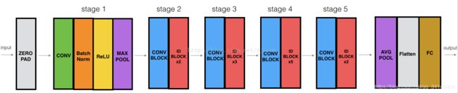
对于ResNet来说,最重要的概念就是残差单元。ResNet相比普通网络每两层间增加了短路机制,将残差加入特征学习。
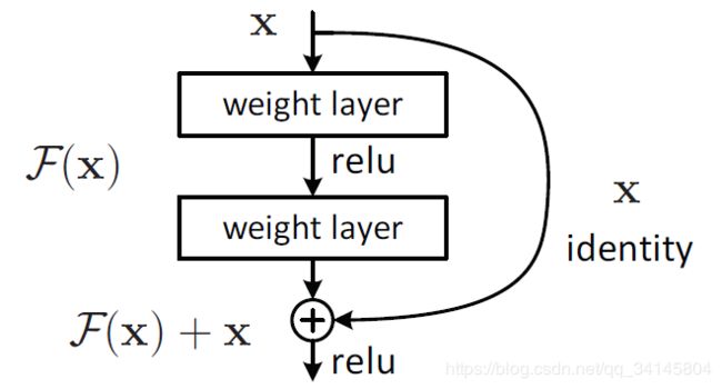
残差单元根据网络深度有两种典型结构。我们使用的ResNet-50网络采用的残差单元是下图右侧这种类型。注意,1x1的卷积可以改变维度,使得短路连接时输入输出的维度一致。

在文件resnet.py中我们基于ResNet-50构造了Faster-RCNN的base网络,代码如下:
from __future__ import print_function
from __future__ import absolute_import

from keras.layers import Input, Add, Dense, Activation, Flatten, Convolution2D, MaxPooling2D, ZeroPadding2D, \
    AveragePooling2D, TimeDistributed

from keras import backend as K

from keras_frcnn.RoiPoolingConv import RoiPoolingConv
from keras_frcnn.FixedBatchNormalization import FixedBatchNormalization
# 默认的模型文件地址
def get_weight_path():
    if K.image_dim_ordering() == 'th':
        return 'resnet50_weights_th_dim_ordering_th_kernels_notop.h5'
    else:
        return 'resnet50_weights_tf_dim_ordering_tf_kernels.h5'
# 根据输入的宽高计算输出的大小
def get_img_output_length(width, height):
    def get_output_length(input_length):
        # zero_pad
        input_length += 6
        # apply 4 strided convolutions
        filter_sizes = [7, 3, 1, 1]
        stride = 2
        for filter_size in filter_sizes:
            input_length = (input_length - filter_size + stride) // stride
        return input_length

    return get_output_length(width), get_output_length(height)
# Identity Block模块,输入和输出相同
def identity_block(input_tensor, kernel_size, filters, stage, block, trainable=True):

    nb_filter1, nb_filter2, nb_filter3 = filters

    if K.image_dim_ordering() == 'tf':
        bn_axis = 3
    else:
        bn_axis = 1

    conv_name_base = 'res' + str(stage) + block + '_branch'
    bn_name_base = 'bn' + str(stage) + block + '_branch'

    x = Convolution2D(nb_filter1, (1, 1), name=conv_name_base + '2a', trainable=trainable)(input_tensor)
    x = FixedBatchNormalization(axis=bn_axis, name=bn_name_base + '2a')(x)
    x = Activation('relu')(x)

    x = Convolution2D(nb_filter2, (kernel_size, kernel_size), padding='same', name=conv_name_base + '2b', trainable=trainable)(x)
    x = FixedBatchNormalization(axis=bn_axis, name=bn_name_base + '2b')(x)
    x = Activation('relu')(x)

    x = Convolution2D(nb_filter3, (1, 1), name=conv_name_base + '2c', trainable=trainable)(x)
    x = FixedBatchNormalization(axis=bn_axis, name=bn_name_base + '2c')(x)

    x = Add()([x, input_tensor])
    x = Activation('relu')(x)
    return x
# Conv Block模块,输入和输出的维度不同。
def conv_block(input_tensor, kernel_size, filters, stage, block, strides=(2, 2), trainable=True):

    nb_filter1, nb_filter2, nb_filter3 = filters
    if K.image_dim_ordering() == 'tf':
        bn_axis = 3
    else:
        bn_axis = 1

    conv_name_base = 'res' + str(stage) + block + '_branch'
    bn_name_base = 'bn' + str(stage) + block + '_branch'

    x = Convolution2D(nb_filter1, (1, 1), strides=strides, name=conv_name_base + '2a', trainable=trainable)(input_tensor)
    x = FixedBatchNormalization(axis=bn_axis, name=bn_name_base + '2a')(x)
    x = Activation('relu')(x)

    x = Convolution2D(nb_filter2, (kernel_size, kernel_size), padding='same', name=conv_name_base + '2b', trainable=trainable)(x)
    x = FixedBatchNormalization(axis=bn_axis, name=bn_name_base + '2b')(x)
    x = Activation('relu')(x)

    x = Convolution2D(nb_filter3, (1, 1), name=conv_name_base + '2c', trainable=trainable)(x)
    x = FixedBatchNormalization(axis=bn_axis, name=bn_name_base + '2c')(x)

    shortcut = Convolution2D(nb_filter3, (1, 1), strides=strides, name=conv_name_base + '1', trainable=trainable)(input_tensor)
    shortcut = FixedBatchNormalization(axis=bn_axis, name=bn_name_base + '1')(shortcut)

    x = Add()([x, shortcut])
    x = Activation('relu')(x)
    return x
# base网络的整体构造
def nn_base(input_tensor=None, trainable=False):

    # Determine proper input shape
    if K.image_dim_ordering() == 'th':
        input_shape = (3, None, None)
    else:
        input_shape = (None, None, 3)

    if input_tensor is None:
        img_input = Input(shape=input_shape) # placeholder
    else:
        if not K.is_keras_tensor(input_tensor):
            img_input = Input(tensor=input_tensor, shape=input_shape)
        else:
            img_input = input_tensor

    if K.image_dim_ordering() == 'tf':
        bn_axis = 3
    else:
        bn_axis = 1
# 用ZeroPadding调整维度
    x = ZeroPadding2D((3, 3))(img_input)

    x = Convolution2D(64, (7, 7), strides=(2, 2), name='conv1', trainable = trainable)(x)
    x = FixedBatchNormalization(axis=bn_axis, name='bn_conv1')(x)
    x = Activation('relu')(x)
    x = MaxPooling2D((3, 3), strides=(2, 2))(x)

    x = conv_block(x, 3, [64, 64, 256], stage=2, block='a', strides=(1, 1), trainable = trainable)
    x = identity_block(x, 3, [64, 64, 256], stage=2, block='b', trainable = trainable)
    x = identity_block(x, 3, [64, 64, 256], stage=2, block='c', trainable = trainable)

    x = conv_block(x, 3, [128, 128, 512], stage=3, block='a', trainable = trainable)
    x = identity_block(x, 3, [128, 128, 512], stage=3, block='b', trainable = trainable)
    x = identity_block(x, 3, [128, 128, 512], stage=3, block='c', trainable = trainable)
    x = identity_block(x, 3, [128, 128, 512], stage=3, block='d', trainable = trainable)

    x = conv_block(x, 3, [256, 256, 1024], stage=4, block='a', trainable = trainable)
    x = identity_block(x, 3, [256, 256, 1024], stage=4, block='b', trainable = trainable)
    x = identity_block(x, 3, [256, 256, 1024], stage=4, block='c', trainable = trainable)
    x = identity_block(x, 3, [256, 256, 1024], stage=4, block='d', trainable = trainable)
    x = identity_block(x, 3, [256, 256, 1024], stage=4, block='e', trainable = trainable)
    x = identity_block(x, 3, [256, 256, 1024], stage=4, block='f', trainable = trainable)

    return x
接着定义了RPN()和Classifier()函数,用base网络的输出作为输入,分别提取RPN和Classifier的分类和回归特征。为了简化网络,我们去除了Classifier中的Timedistributed层。
def rpn(base_layers,num_anchors):

    x = Convolution2D(512, (3, 3), padding='same', activation='relu', kernel_initializer='normal', name='rpn_conv1')(base_layers) # output of base_layers

    x_class = Convolution2D(num_anchors, (1, 1), activation='sigmoid', kernel_initializer='uniform', name='rpn_out_class')(x)
    x_regr = Convolution2D(num_anchors * 4, (1, 1), activation='linear', kernel_initializer='zero', name='rpn_out_regress')(x)

    return [x_class, x_regr, base_layers]

def classifier_layers(x, input_shape, trainable=False):

        if K.backend() == 'tensorflow':
        x = conv_block(x, 3, [512, 512, 2048], stage=5, block='a', input_shape=input_shape, strides=(2, 2), trainable=trainable)
    elif K.backend() == 'theano':
        x = conv_block(x, 3, [512, 512, 2048], stage=5, block='a', input_shape=input_shape, strides=(1, 1), trainable=trainable)

    x = identity_block(x, 3, [512, 512, 2048], stage=5, block='b', trainable=trainable)
    x = identity_block(x, 3, [512, 512, 2048], stage=5, block='c', trainable=trainable)
    x = AveragePooling2D((7, 7), name='avg_pool')(x)

    return x

def classifier(base_layers, input_rois, num_rois, nb_classes = 21, trainable=False):

    if K.backend() == 'tensorflow':
        pooling_regions = 14
        input_shape = (num_rois,14,14,1024)
    elif K.backend() == 'theano':
        pooling_regions = 7
        input_shape = (num_rois,1024,7,7)

    out_roi_pool = RoiPoolingConv(pooling_regions, num_rois)([base_layers, input_rois])
    out = classifier_layers(out_roi_pool, input_shape=input_shape, trainable=True)

    out = Flatten()(out)

    out_class = Dense(nb_classes, activation='softmax', kernel_initializer='zero', name='dense_class_{}'.format(nb_classes)(out)
    # note: no regression target for bg class
    out_regr = Dense(4 * (nb_classes-1), activation='linear', kernel_initializer='zero', name='dense_regress_{}'.format(nb_classes)(out)
    return [out_class, out_regr]
对于RPN来说,每一个输入的点都对应num_anchor个输出。其中x_class经过二分类输出当前的框中有目标物体的概率;x_regr输出框的坐标。RoiPoolingConv是一个自定义的层。参数包括池化核大小pool_size和每次处理的roi个数num_rois。输入是base网络输出的特征图张量,其中一个形式为(1,rows,cols,channels),1个为(1,num_rois,4)。输出是经过RoiPooling的标准大小的特征,形式为(1,num_rois,channels,pool_size,pool_size)的张量。
RPN的思想和实现
RPN的思路是将上一步提取出的特征图映射到原图,从而将生成的框与原图中的ground truth进行IOU的计算,判断匹配的程度。满足一定条件时就对框进行初步的回归。对于Faster-RCNN来说,也就是将特征图的每一个点作为一个锚点,生成num_anchor个尺度不同的Anchor。由于尺度是设定好的,这样做就避免了多次放缩造成的浪费,提高了检测效率。这一部分的代码如下:
from __future__ import absolute_import

import numpy as np

import cv2

import random

import copy

# 这里C代表一个参数类(上面的Config),C = Config()

def calc_rpn(C, img_data, width, height, resized_width, resized_height, img_length_calc_function):


    # 接下来读取了几个参数,downscale就是从图片到特征图的缩放倍数(默认为16.0) 这里,

    # img_length_calc_function(也就是实际的resnet中的get_img_output_length中整除的值一样。)

    # anchor_size和anchor_ratios是我们初步选区大小的参数,比如3个size和3个ratios,可以组合成9种不同形状大小的选区。

    downscale = float(C.rpn_stride)

    anchor_sizes = C.anchor_box_scales

    anchor_ratios = C.anchor_box_ratios

    num_anchors = len(anchor_sizes) * len(anchor_ratios)


    # calculate the output map size based on the network architecture

    # 接下来,

    # 通过img_length_calc_function 对VGG16 返回的是一个height和width都整除16的结果这个方法计算出了特征图的尺寸。

    # output_width = output_height = 600 // 16 = 37

    (output_width, output_height) = img_length_calc_function(resized_width, resized_height)


    # 下一步是几个变量初始化可以先不看,后面用到的时候再看。


    # n_anchratios = 3

    n_anchratios = len(anchor_ratios)


    # initialise empty output objectives

    y_rpn_overlap = np.zeros((output_height, output_width, num_anchors))

    y_is_box_valid = np.zeros((output_height, output_width, num_anchors))

    y_rpn_regr = np.zeros((output_height, output_width, num_anchors * 4))


    num_bboxes = len(img_data['bboxes'])


    num_anchors_for_bbox = np.zeros(num_bboxes).astype(int)

    best_anchor_for_bbox = -1*np.ones((num_bboxes, 4)).astype(int)

    best_iou_for_bbox = np.zeros(num_bboxes).astype(np.float32)

    best_x_for_bbox = np.zeros((num_bboxes, 4)).astype(int)

    best_dx_for_bbox = np.zeros((num_bboxes, 4)).astype(np.float32)


    # 因为我们的计算都是基于resize以后的图像的,所以接下来把bbox中的x1,x2,y1,y2分别通过缩放匹配到resize以后的图像。

    # 这里记做gta,尺寸为(num_of_bbox,4)。

    # get the GT box coordinates, and resize to account for image resizing

    gta = np.zeros((num_bboxes, 4))

    for bbox_num, bbox in enumerate(img_data['bboxes']):

        # get the GT box coordinates, and resize to account for image resizing

        gta[bbox_num, 0] = bbox['x1'] * (resized_width / float(width))

        gta[bbox_num, 1] = bbox['x2'] * (resized_width / float(width))

        gta[bbox_num, 2] = bbox['y1'] * (resized_height / float(height))

        gta[bbox_num, 3] = bbox['y2'] * (resized_height / float(height))


    # rpn ground truth

    # 这一段计算了anchor的长宽,然后比较重要的就是把特征图的每一个点作为一个锚点,

    # 通过乘以downscale,映射到图片的实际尺寸,再结合anchor的尺寸,忽略掉超出图片范围的。

    # 一个个大小、比例不一的矩形选框就跃然纸上了。

    # 第一层for 3层

    # 第二层for 3层

    for anchor_size_idx in range(len(anchor_sizes)):

        for anchor_ratio_idx in range(n_anchratios):

            # 框的尺寸选定

            anchor_x = anchor_sizes[anchor_size_idx] * anchor_ratios[anchor_ratio_idx][0]

            anchor_y = anchor_sizes[anchor_size_idx] * anchor_ratios[anchor_ratio_idx][1]

            # 对1024 --> 600 --> 37的形式,output_width = 37

            # 选定锚点坐标: x_anc y_anc

            for ix in range(output_width):

                # x-coordinates of the current anchor box

                x1_anc = downscale * (ix + 0.5) - anchor_x / 2

                x2_anc = downscale * (ix + 0.5) + anchor_x / 2


                # ignore boxes that go across image boundaries

                if x1_anc < 0 or x2_anc > resized_width:

                    continue


                for jy in range(output_height):


                    # y-coordinates of the current anchor box

                    y1_anc = downscale * (jy + 0.5) - anchor_y / 2

                    y2_anc = downscale * (jy + 0.5) + anchor_y / 2


                    # ignore boxes that go across image boundaries

                    if y1_anc < 0 or y2_anc > resized_height:

                        continue


                    # 定义了两个变量,bbox_type和best_iou_for_loc,后面会用到。计算了anchor与gta的交集 iou(),

                    # 然后就是如果交集大于best_iou_for_bbox[bbox_num]或者大于我们设定的阈值,就会去计算gta和anchor的中心点坐标,

                    # bbox_type indicates whether an anchor should be a target

                    bbox_type = 'neg'


                    # this is the best IOU for the (x,y) coord and the current anchor

                    # note that this is different from the best IOU for a GT bbox

                    best_iou_for_loc = 0.0


                    # 对选出的选择框,判断其和实际上图片的所有Bbox中,有无满足大于规定threshold的情况。

                    for bbox_num in range(num_bboxes):


                        # get IOU of the current GT box and the current anchor box

                        curr_iou = iou([gta[bbox_num, 0], gta[bbox_num, 2], gta[bbox_num, 1], gta[bbox_num, 3]], [x1_anc, y1_anc, x2_anc, y2_anc])

                        # calculate the regression targets if they will be needed

                        # 默认的最大rpn重叠部分(rpn_max_overlap)为0.7,最小(rpn_min_overlap)为0.3

                        if curr_iou > best_iou_for_bbox[bbox_num] or curr_iou > C.rpn_max_overlap:

                            cx = (gta[bbox_num, 0] + gta[bbox_num, 1]) / 2.0

                            cy = (gta[bbox_num, 2] + gta[bbox_num, 3]) / 2.0

                            cxa = (x1_anc + x2_anc)/2.0

                            cya = (y1_anc + y2_anc)/2.0


                            # 计算出x,y,w,h四个值的梯度值。

                            # 为什么要计算这个梯度呢?因为RPN计算出来的区域不一定是很准确的,从只有9个尺寸的anchor也可以推测出来,

                            # 因此我们在预测时还会进行一次回归计算,而不是直接使用这个区域的坐标。

                            tx = (cx - cxa) / (x2_anc - x1_anc)

                            ty = (cy - cya) / (y2_anc - y1_anc)

                            tw = np.log((gta[bbox_num, 1] - gta[bbox_num, 0]) / (x2_anc - x1_anc))

                            th = np.log((gta[bbox_num, 3] - gta[bbox_num, 2]) / (y2_anc - y1_anc))


                        # 前提是:当前的bbox不是背景 != 'bg'

                        if img_data['bboxes'][bbox_num]['class'] != 'bg':


                            # all GT boxes should be mapped to an anchor box, so we keep track of which anchor box was best

                            if curr_iou > best_iou_for_bbox[bbox_num]:

                                # jy 高度 ix 宽度

                                best_anchor_for_bbox[bbox_num] = [jy, ix, anchor_ratio_idx, anchor_size_idx]

                                best_iou_for_bbox[bbox_num] = curr_iou

                                best_x_for_bbox[bbox_num,:] = [x1_anc, x2_anc, y1_anc, y2_anc]

                                best_dx_for_bbox[bbox_num,:] = [tx, ty, tw, th]


                            # we set the anchor to positive if the IOU is >0.7 (it does not matter if there was another better box, it just indicates overlap)

                            if curr_iou > C.rpn_max_overlap:

                                bbox_type = 'pos'

                                # 因为num_anchors_for_bbox 形式为 [0, 0, 0, 0]

                                # 这步操作的结果为 [1, 1, 1, 1]

                                num_anchors_for_bbox[bbox_num] += 1

                                # we update the regression layer target if this IOU is the best for the current (x,y) and anchor position

                                if curr_iou > best_iou_for_loc:

                                    # 不断修正最佳iou对应的区域和梯度

                                    best_iou_for_loc = curr_iou

                                    best_grad = (tx, ty, tw, th)


                            # if the IOU is >0.3 and <0.7, it is ambiguous and no included in the objective

                            if C.rpn_min_overlap < curr_iou < C.rpn_max_overlap:

                                # gray zone between neg and pos

                                if bbox_type != 'pos':

                                    bbox_type = 'neutral'


                    # turn on or off outputs depending on IOUs

                    # 接下来根据bbox_type对本anchor进行打标,y_is_box_valid和y_rpn_overlap分别定义了这个anchor是否可用和是否包含对象。

                    if bbox_type == 'neg':

                        y_is_box_valid[jy, ix, anchor_ratio_idx + n_anchratios * anchor_size_idx] = 1

                        y_rpn_overlap[jy, ix, anchor_ratio_idx + n_anchratios * anchor_size_idx] = 0

                    elif bbox_type == 'neutral':

                        y_is_box_valid[jy, ix, anchor_ratio_idx + n_anchratios * anchor_size_idx] = 0

                        y_rpn_overlap[jy, ix, anchor_ratio_idx + n_anchratios * anchor_size_idx] = 0

                    elif bbox_type == 'pos':

                        y_is_box_valid[jy, ix, anchor_ratio_idx + n_anchratios * anchor_size_idx] = 1

                        y_rpn_overlap[jy, ix, anchor_ratio_idx + n_anchratios * anchor_size_idx] = 1

                        # 默认是36个选择

                        start = 4 * (anchor_ratio_idx + n_anchratios * anchor_size_idx)

                        y_rpn_regr[jy, ix, start:start+4] = best_grad


    # we ensure that every bbox has at least one positive RPN region

    # 这里又出现了一个潜在问题: 可能会有bbox可能找不到心仪的anchor,那这些训练数据就没法利用了,

    # 因此我们用一个折中的办法来保证每个bbox至少有一个anchor与之对应。

    # 下面是具体的方法,比较简单,对于没有对应anchor的bbox,在中性anchor里挑最好的,当然前提是你不能跟我完全不相交,那就太过分了。。

    for idx in range(num_anchors_for_bbox.shape[0]):

        if num_anchors_for_bbox[idx] == 0:

            # no box with an IOU greater than zero ... 遇到这种情况只能pass了

            if best_anchor_for_bbox[idx, 0] == -1:

                continue

            y_is_box_valid[

                best_anchor_for_bbox[idx,0], best_anchor_for_bbox[idx,1], best_anchor_for_bbox[idx,2] + n_anchratios *

                best_anchor_for_bbox[idx,3]] = 1

            y_rpn_overlap[

                best_anchor_for_bbox[idx,0], best_anchor_for_bbox[idx,1], best_anchor_for_bbox[idx,2] + n_anchratios *

                best_anchor_for_bbox[idx,3]] = 1

            start = 4 * (best_anchor_for_bbox[idx,2] + n_anchratios * best_anchor_for_bbox[idx,3])

            y_rpn_regr[

                best_anchor_for_bbox[idx,0], best_anchor_for_bbox[idx,1], start:start+4] = best_dx_for_bbox[idx, :]


    # y_rpn_overlap 原来的形式np.zeros((output_height, output_width, num_anchors))

    # 现在变为 (num_anchors, output_height, output_width)

    y_rpn_overlap = np.transpose(y_rpn_overlap, (2, 0, 1))

    # (新的一列,num_anchors, output_height, output_width)

    y_rpn_overlap = np.expand_dims(y_rpn_overlap, axis=0)


    y_is_box_valid = np.transpose(y_is_box_valid, (2, 0, 1))

    y_is_box_valid = np.expand_dims(y_is_box_valid, axis=0)


    y_rpn_regr = np.transpose(y_rpn_regr, (2, 0, 1))

    y_rpn_regr = np.expand_dims(y_rpn_regr, axis=0)


    # pos表示box neg表示背景

    pos_locs = np.where(np.logical_and(y_rpn_overlap[0, :, :, :] == 1, y_is_box_valid[0, :, :, :] == 1))

    neg_locs = np.where(np.logical_and(y_rpn_overlap[0, :, :, :] == 0, y_is_box_valid[0, :, :, :] == 1))


    num_pos = len(pos_locs[0])


    # one issue is that the RPN has many more negative than positive regions, so we turn off some of the negative

    # regions. We also limit it to 256 regions.

    # 因为negtive的anchor肯定远多于postive的,

    # 因此在这里设定了regions数量的最大值为256,并对pos和neg的样本进行了均匀的取样。

    num_regions = 256


    # 对感兴趣的框超过128的时候...

    if len(pos_locs[0]) > num_regions/2:

        # val_locs为一个list

        val_locs = random.sample(range(len(pos_locs[0])), len(pos_locs[0]) - num_regions/2)

        y_is_box_valid[0, pos_locs[0][val_locs], pos_locs[1][val_locs], pos_locs[2][val_locs]] = 0

        num_pos = num_regions/2

    # 使得neg(背景)和pos(锚框)数量一致

    if len(neg_locs[0]) + num_pos > num_regions:

        val_locs = random.sample(range(len(neg_locs[0])), len(neg_locs[0]) - num_pos)

        y_is_box_valid[0, neg_locs[0][val_locs], neg_locs[1][val_locs], neg_locs[2][val_locs]] = 0


    y_rpn_cls = np.concatenate([y_is_box_valid, y_rpn_overlap], axis=1)

    y_rpn_regr = np.concatenate([np.repeat(y_rpn_overlap, 4, axis=1), y_rpn_regr], axis=1)

    # 最后,得到了两个返回值y_rpn_cls,y_rpn_regr。分别用于确定anchor是否包含物体,和回归梯度。

    # 值得注意的是, y_rpn_cls和y_rpn_regr数量是比实际的输入图片对应的Bbox数量多挺多的。

    return np.copy(y_rpn_cls), np.copy(y_rpn_regr)
生成RPN这一步骤的关键在于用多个for循环不断地选择和匹配anchor box与ground truth的bounding box。这样一个多对多的过程可以筛选掉过多的anchor box并保证每个bbox有至少一个anchor box与之匹配。
从RPN到ROI
这一步是由rpn_to_roi和calc_iou两个函数实现的。rpn_to_roi主要作用是非极大值抑制,对重叠的rpn框进行筛选,使它们的数量进一步减少,得到roi。而calc_iou的作用是,通过calc_iou()找出剩下的不多的roi对应ground truth里重合度最高的bbox,从而获得model_classifier的数据和标签。
import numpy as np
import pdb
import math
from . import data_generators
import copy


def calc_iou(R, img_data, C, class_mapping):

	bboxes = img_data['bboxes']
	(width, height) = (img_data['width'], img_data['height'])
	# 获取resize后的原图尺度
	(resized_width, resized_height) = data_generators.get_new_img_size(width, height, C.im_size)

	gta = np.zeros((len(bboxes), 4))
        # 计算resize后的bounding box坐标
	for bbox_num, bbox in enumerate(bboxes):

		gta[bbox_num, 0] = int(round(bbox['x1'] * (resized_width / float(width))/C.rpn_stride))
		gta[bbox_num, 1] = int(round(bbox['x2'] * (resized_width / float(width))/C.rpn_stride))
		gta[bbox_num, 2] = int(round(bbox['y1'] * (resized_height / float(height))/C.rpn_stride))
		gta[bbox_num, 3] = int(round(bbox['y2'] * (resized_height / float(height))/C.rpn_stride))

	x_roi = []
	y_class_num = []
	y_class_regr_coords = []
	y_class_regr_label = []
	IoUs = []
        # R = [boxes, probs]
        # 计算每个roi的坐标
	for ix in range(R.shape[0]):
		(x1, y1, x2, y2) = R[ix, :]
		x1 = int(round(x1))
		y1 = int(round(y1))
		x2 = int(round(x2))
		y2 = int(round(y2))

		best_iou = 0.0
		best_bbox = -1
                # 计算每个roi最匹配的bbox
		for bbox_num in range(len(bboxes)):
			curr_iou = data_generators.iou([gta[bbox_num, 0], gta[bbox_num, 2], gta[bbox_num, 1], gta[bbox_num, 3]], [x1, y1, x2, y2])
			if curr_iou > best_iou:
				best_iou = curr_iou
				best_bbox = bbox_num
                # 如果所有bbox与该roi的IOU小于最小值,则该roi被舍去。
		if best_iou < C.classifier_min_overlap:
				continue
		else: # 否则采用
			w = x2 - x1
			h = y2 - y1
			x_roi.append([x1, y1, w, h])
			IoUs.append(best_iou)
                        # 如果所有的bbox与该rois的IOU都介于最小值和最大值之间,则为背景类。
			if C.classifier_min_overlap <= best_iou < C.classifier_max_overlap:
				cls_name = 'bg'
                        # 如果有一个bbox与该rois匹配度高,则为正类。
			elif C.classifier_max_overlap <= best_iou:
				cls_name = bboxes[best_bbox]['class']
                                # 该bbox的中心点坐标
				cxg = (gta[best_bbox, 0] + gta[best_bbox, 1]) / 2.0
				cyg = (gta[best_bbox, 2] + gta[best_bbox, 3]) / 2.0
                                # rois的中心点坐标
				cx = x1 + w / 2.0
				cy = y1 + h / 2.0
                                # 反向传播
				tx = (cxg - cx) / float(w)
				ty = (cyg - cy) / float(h)
				tw = np.log((gta[best_bbox, 1] - gta[best_bbox, 0]) / float(w))
				th = np.log((gta[best_bbox, 3] - gta[best_bbox, 2]) / float(h))
			else:
				print('roi = {}'.format(best_iou))
				raise RuntimeError

		class_num = class_mapping[cls_name] # 取类型编号
		class_label = len(class_mapping) * [0]
		class_label[class_num] = 1          # 0-1标签
		y_class_num.append(copy.deepcopy(class_label))
		coords = [0] * 4 * (len(class_mapping) - 1)
		labels = [0] * 4 * (len(class_mapping) - 1)
                # 坐标和类别的标签
		if cls_name != 'bg':
			label_pos = 4 * class_num
			sx, sy, sw, sh = C.classifier_regr_std
                        # 回归坐标
			coords[label_pos:4+label_pos] = [sx*tx, sy*ty, sw*tw, sh*th]
			labels[label_pos:4+label_pos] = [1, 1, 1, 1]
			y_class_regr_coords.append(copy.deepcopy(coords))
			y_class_regr_label.append(copy.deepcopy(labels)) 		else:
			y_class_regr_coords.append(copy.deepcopy(coords))
			y_class_regr_label.append(copy.deepcopy(labels)) # 背景类标签全0

	if len(x_roi) == 0:
		return None, None, None, None

	X = np.array(x_roi) # bbox
	Y1 = np.array(y_class_num) # one-hot类别标签
	Y2 = np.concatenate([np.array(y_class_regr_label),np.array(y_class_regr_coords)],axis=1) # 类别和回归坐标的标签
        # np.expand_dims:增加一个通道
	return np.expand_dims(X, axis=0), np.expand_dims(Y1, axis=0), np.expand_dims(Y2, axis=0), IoUs
X保留所有的背景和正类bbox的roi框; Y1 是类别one-hot转码; Y2是对应类别的标签及回归要学习的坐标位置; IouS只用于debug。
训练过程
Faster-RCNN总共有4个损失函数,分别是RPN到ROI阶段的两个,即函数calc_rpn的两个输出:y_rpn_cls(RPN是否包含物体)和y_rpn_regr(RPN的回归坐标);ROI到bbox阶段的两个,即函数calc_iou的输出:y_class_regr_label(最终输出的物体类型)和y_class_regr_coords(最终输出的bbox)。四个损失函数分成了两个RPN和Classifier两个模型来训练。
抛开上面这些bounding box的选择和回归操作,训练过程和之前介绍过的分类网络是类似的。优化器和训练过程的超参数如下:
optimizer = Adam(lr=1e-5)
optimizer_classifier = Adam(lr=1e-5)
model_rpn.compile(optimizer=optimizer, loss=[losses.rpn_loss_cls(num_anchors), losses.rpn_loss_regr(num_anchors)])
model_classifier.compile(optimizer=optimizer_classifier, loss=[losses.class_loss_cls, losses.class_loss_regr(len(classes_count)-1)], metrics={'dense_class_{}'.format(len(classes_count)): 'accuracy'})
model_all.compile(optimizer='sgd', loss='mae')

epoch_length = 300
num_epochs = int(options.num_epochs)
iter_num = 0
采用了train_on_batch函数来训练模型。每训练完一个batch就输出四个损失函数的大小。每个epoch结束输出在验证集上的准确率。假设batch_size=300,epoch_num=20,训练结果如图
train_frcnn.py文件会将训练得到的权重保存为hdf5文件,路径C.model_path见config.py文件。
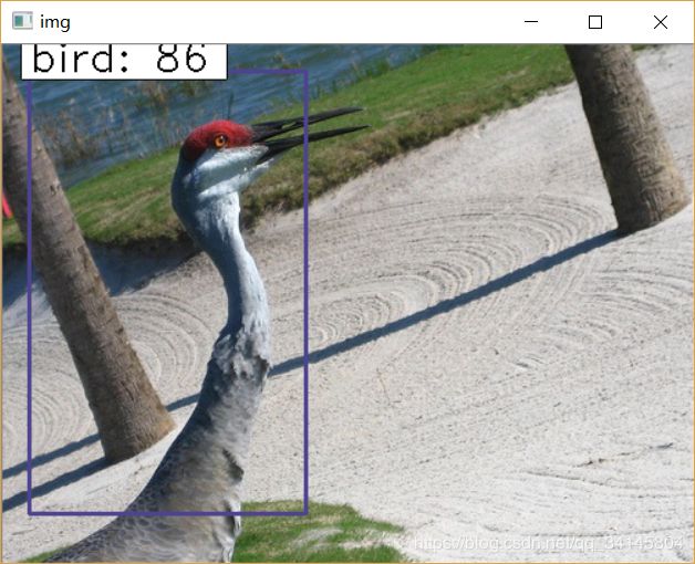
测试
在test_frcnn.py文件中指定测试图片的位置,程序从默认路径载入训练好的权重,结果如图: