数字图像处理与Python实现笔记之彩色图像处理初步

摘要

1. 简要介绍数字图像处理涉及的一些基本概念、基本运算、基本类型，以及如何通过Python对数字图像进行读取和简单操作。
2. 以彩色图像为例对数字图像处理的基本操作进行介绍，熟悉数字图像处理的基本过程，主要包括颜色空间的基本概念、伪彩色图像处理操作，彩色图像处理简单操作。
3. 瞄准在空间域中对图像进行增强，介绍空间滤波的机理、基本概念以及使用的基本技术。本章内容包括空间滤波基本概念、基于空间滤波的图像平滑处理、基于空间滤波的锐化操作以及混合空间增强。
4. 从频域角度入手对图像处理及增强方法展开介绍。因为频域滤波所需的数学知识较多，所以本章采取由浅入深的策略，首先介绍一维傅里叶变换，其次介绍二维傅里叶变换和快速傅里叶变换，最后介绍图像频域滤波中出现的各种技术，其大体可分为低通滤波和高通滤波两大类。
5. 从全局特征提取和局部特征提取两方面入手，分别介绍颜色特征、纹理特征、形状特征、边缘特征、点特征的提取方法。本章内容是目前机器视觉和图像处理领域的学者关注较多的内容，通过穿插较多的实例，帮助读者理解图像特征提取的基本技术。
6. 瞄准如何减少图像传输及存储数据大小，介绍主要使用的压缩技术，包括有损压缩和无损压缩等，并使用JPEG压缩技术串讲全章知识点。
7. 介绍图像的小波域表示及多分辨率表示。

绪论

• 人工智能是引领未来发展的战略性技术，是新一轮科技革命和产业变革的重要驱动力量，将深刻地改变人类社会生活。

• 促进人工智能和实体经济的深度融合，构建数据驱动、人机协同、跨界融合、共创分享的智能经济形态，更是推动质量变革、效率变革、动力变革的重要途经。

• 进年来，我国人工智能新技术、新产品、新业态持续涌现，与农业、制造业、服务业等行业的融合步伐明显加快，在技术创新、应用推广、产业发展等方面成效初显。

• 人工智能技术并不是一个新生事物，它在最近几年引起全球性关注并得到飞速发展的主要原因，在于它的三个基本要素（算法、数据、算力）的迅猛发展，其中又以数据和算力的发展尤为重要。

• 物联网技术的蓬勃发展使得数据累计的难度越来越低，而芯片算力的不断提升，使得过去只能通过云计算才能完成的人工智能运算，现在可以下沉到最普通的设备上完成。

• 物联网技术为机器带来感知能力，而人工智能则通过计算算力为机器带来了决策能力，正如感知和大脑对自然生命进化所起到的必然性作用。

1 数字图像处理基础知识

https://hulin.blog.csdn.net/article/details/107570020

2 彩色图像处理初步

• 对于灰度图像而言，其每个像素的亮度用一个数值表示即可。而彩色图像的每个像素包含了颜色信息，每个像素的光强度和色度需用三个数值描述。
• 研究彩色图像的主要原因：第一，彩色图像符合人类视觉特点，人类可以辨别几千种颜色色调和亮度，但却只能辨别几十种灰度层次。第二，彩色可以更好的表达图像的特征，可根据图像的颜色特征简化目标物的区分与识别。

2.1 彩色图像的颜色空间

• 彩色图像的颜色空间也称为颜色模型和彩色系统，用于对颜色进行描述和说明。常用的颜色空间包括RGB颜色空间和HSI颜色空间。

2.1.1　RGB颜色空间

-　白光通过玻璃棱镜会出现紫色到红色的连续彩色光谱，光由多种色谱构成。

• 人眼中有大量对红、绿、蓝颜色敏感的追状体细胞，因此常用RGB颜色空间表达彩色图像信息。这3种原色的混合色基本覆盖了人类的色彩空间，从而满足了人类的色彩体验。
• RGB图像由三个图像分量组成，分别是R通道图像、G通道图像和B通道图像。

import skimage.data as data
import matplotlib.pyplot as plt

image = data.coffee()  # 载入RGB图像
fig = plt.figure()
plt.axis('off')  # 不显示坐标轴
plt.imshow(image)  # 显示RGB彩色图像

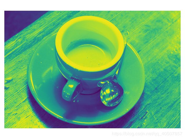
# R 通道图像
imageR = image[:, :, 0]
plt.figure()
plt.axis('off')  # 不显示坐标轴
plt.imshow(imageR, cmap='gray')

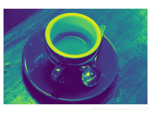
# G 通道图像
imageG = image[:, :, 1]
plt.figure()
plt.axis('off')  # 不显示坐标轴
plt.imshow(imageG, cmap='gray')

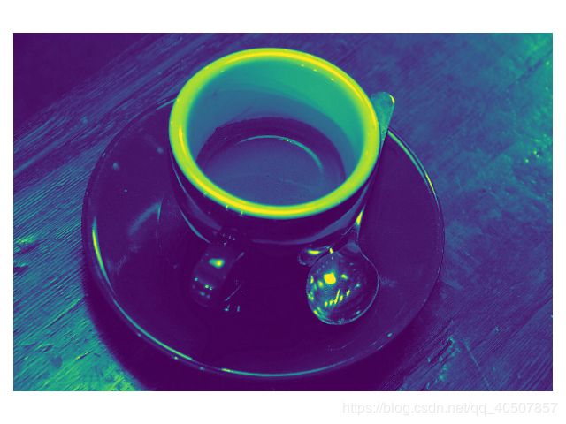
# B 通道图像
imageB = image[:, :, 2]
plt.figure()
plt.axis('off')  # 不显示坐标轴
plt.imshow(imageB, cmap='gray')

plt.show()

• R 通道图像
  

• G 通道图像
  

• B 通道图像
  

2.1.2　HSI颜色空间

• HSI颜色空间接近人类视觉感知颜色的方式，包含三个分量分别是：色调（Hue，H），饱和度（Saturation，S），亮度（Intensity，I）
  
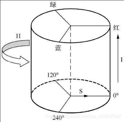
• HSI颜色空间圆柱体的横截面称为色环，色环更加清晰的展示了色调和饱和度两个参数
  
• 色调H由角度表示，其颜色表示最接近哪个光谱波长。
• 饱和度S由色环的圆心到颜色点的半径表示，距离越长表示饱和度越高，颜色越鲜明。
• 亮度I由颜色点到圆柱底部的距离表示。
• 圆柱体底部圆心表示黑色，顶部圆心表示白色。

2.1.3　RGB和HSI颜色空间的转换

• RGB转到HSI颜色空间：将图像的R、G、B分量分别进行归一化处理

from skimage import data, io
from matplotlib import pyplot as plt
import math
import numpy as np
import sys


def RGB_to_HSI(r, g, b):
    r = r / 255
    g = g / 255
    b = b / 255
    num = 0.5 * ((r - g) + (r - b))
    den = ((r - g) * (r - g) + (r - b) * (g - b)) ** 0.5
    if b <= g:
        if den == 0:
            den = sys.float_info.min
        h = math.acos(num / den)
    elif b > g:
        if den == 0:
            den = sys.float_info.min
        h = (2 * math.pi) - math.acos(num / den)
    s = 1 - (3 * min(r, g, b) / (r + g + b))
    i = (r + g + b) / 3
    return int(h), int(s * 100), int(i * 255)


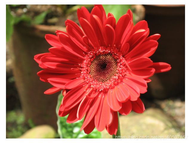
image = io.imread('Red-Flower.jpg')
hsi_image = np.zeros(image.shape, dtype='uint8')
for i in range(image.shape[0]):
    for j in range(image.shape[1]):
        r, g, b = image[i, j, :]
        h, s, i = RGB_to_HSI(r, g, b)
        hsi_image[i, j, :] = (h, s, i)
        print(hsi_image[i, j, :])
plt.figure()
plt.axis('off')
plt.imshow(image)  # 显示RGB原图像

plt.figure()
plt.axis('off')
plt.imshow(image[:, :, 0], cmap='gray')  # 显示RGB原图像R分量

plt.figure()
plt.axis('off')
plt.imshow(image[:, :, 1], cmap='gray')  # 显示RGB原图像G分量

plt.figure()
plt.axis('off')
plt.imshow(image[:, :, 2], cmap='gray')  # 显示RGB原图像B分量

plt.figure()
plt.axis('off')
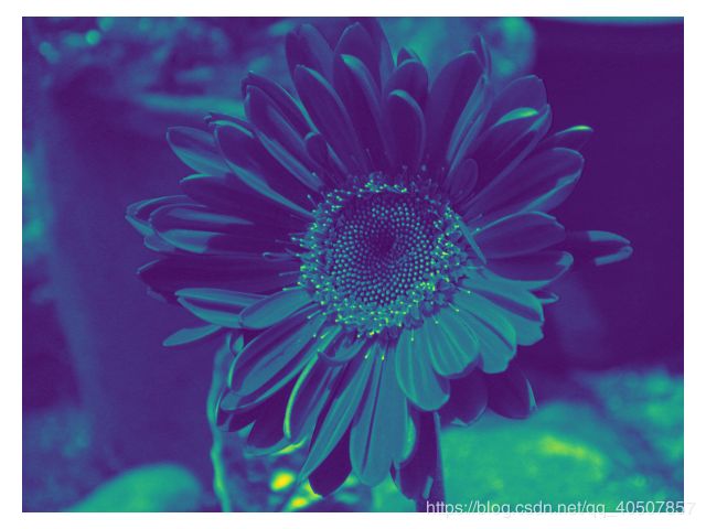
plt.imshow(hsi_image)  # 显示HSI图像

plt.figure()
plt.axis('off')
plt.imshow(hsi_image[:, :, 0], cmap='gray')  # 显示HSI图像H分量

plt.figure()
plt.axis('off')
plt.imshow(hsi_image[:, :, 1], cmap='gray')  # 显示HSI图像S分量

plt.figure()
plt.axis('off')
plt.imshow(hsi_image[:, :, 2], cmap='gray')  # 显示HSI图像I分量

plt.show()

• HSI转到RGB颜色空间

2.2 伪彩色图像处理

• 彩色图像处理可以分为全彩色图像处理和伪彩色图像处理。
• 全彩色图像由全彩色传感器获取，如数码相机和彩色扫描仪。
• 全彩色图像处理方法分为两大类：① 分别处理每一分量图像，然后将处理后的分量图像合成彩色图像。② 直接对彩色像素进行处理。
• 伪彩色图像处理根据一定的规则对灰度值赋以彩色，将灰度图像转化为给定彩色分布的图像。主要包括强度分层技术和灰度值到彩色变换技术。

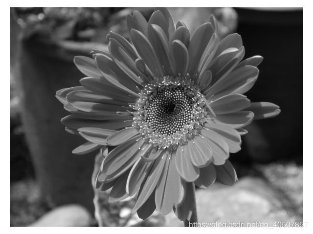
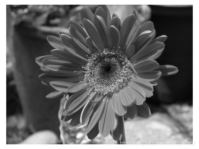
2.2.1 强度分层

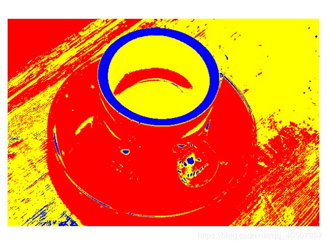
• 强度分层也称为灰度分层或灰度分割。将灰度图像按照灰度值范围划分为不同的层级，然后给每个层级赋予不同的颜色，从而增强不同层级的对比度。强度分层技术将灰度图像转换为伪彩色图像，且伪彩色图像的颜色种类数目与强度分层的数目一致。

• 灰度图像
  

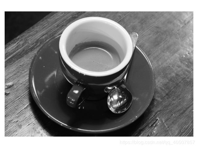
• 强度分层图像
  

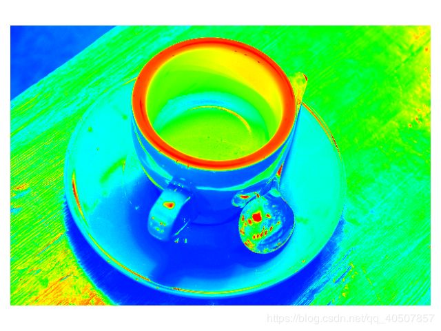
2.2.2 灰度值到彩色变换

• 首先对任何像素的灰度值进行3个独立的变换，然后将3个变换的结果分别作为伪彩色图像的红、绿、蓝通道的亮度值。
• 与强度分层技术相比，灰度值到彩色变换更通用。
• 绘制灰度值到彩色变换的映射关系的代码如下。

from skimage import data, color
from matplotlib import pyplot as plt
import numpy as np

L = 255


# 定义灰度值到彩色变换
def getR(gray):
    if gray < L / 2:
        return 0
    elif gray > L / 4 * 3:
        return L
    else:
        return 4 * gray - 2 * L


def getG(gray):
    if gray < L / 4:
        return 4 * gray
    elif gray > L / 4 * 3:
        return 4 * L - 4 * gray
    return L


def getB(gray):
    if gray < L / 4:
        return L
    elif gray > L / 2:
        return 0
    else:
        return 2 * L - 4 * gray


# 设置字体格式
plt.rcParams['font.sans-serif'] = ['SimHei']
plt.rcParams['font.size'] = 15
plt.rcParams['axes.unicode_minus'] = False
x = [0, 64, 127, 191, 255]

# 绘制灰度图像到R通道的映射关系
plt.figure()
R = []
for i in x:
    R.append(getR(i))
plt.plot(x, R, 'r', label='红色变换')
plt.legend(loc='best')

# 绘制灰度图像到R通道的映射关系
plt.figure()
G = []
for i in x:
    G.append(getG(i))
plt.plot(x, G, 'g', label='绿色变换')
plt.legend(loc='best')

# 绘制灰度图像到B通道的映射关系
plt.figure()
B = []
for i in x:
    B.append(getB(i))
plt.plot(x, B, 'b', marker='o', markersize='5', label='绿色变换')
plt.legend(loc='best')

# 绘制灰度图像到RGB的映射关系
plt.figure()
plt.plot(x, R, 'r')
plt.plot(x, G, 'g')
plt.plot(x, B, 'b', marker='o', markersize='5')

plt.show()

• 灰度图像按以上映射关系转换为彩色图像的代码如下。

from skimage import data, color
from matplotlib import pyplot as plt
import numpy as np

L = 255


# 定义灰度值到彩色变换
def getR(gray):
    if gray < L / 2:
        return 0
    elif gray > L / 4 * 3:
        return L
    else:
        return 4 * gray - 2 * L


def getG(gray):
    if gray < L / 4:
        return 4 * gray
    elif gray > L / 4 * 3:
        return 4 * L - 4 * gray
    return L


def getB(gray):
    if gray < L / 4:
        return L
    elif gray > L / 2:
        return 0
    else:
        return 2 * L - 4 * gray


img = data.coffee()
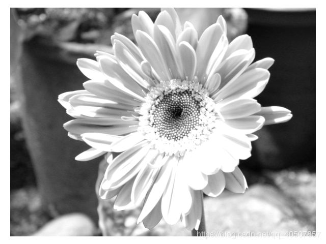
gray_img = color.rgb2gray(img) * 255
color_img = np.zeros(img.shape, dtype='uint8')
for i in range(img.shape[0]):
    for j in range(img.shape[1]):
        r, g, b = getR(gray_img[i, j]), getG(gray_img[i, j]), getB(gray_img[i, j])
        color_img[i, j, :] = (r, g, b)

plt.figure()
plt.axis('off')
plt.imshow(gray_img)

plt.figure()
plt.axis('off')
plt.imshow(color_img)

plt.show()

2.3 基于彩色的图像分割

• 图像分割是把图像分成各具特性的区域并提取出感兴趣区域的技术和过程。
• 基于彩色的图像分割是在颜色空间中进行图像分割
• 基于彩色的图像分割首先观察原始彩色图像的各个分量图像，利用分量图像中感兴趣区域的特征对感兴趣区域进行提取，并弱化背景区域。

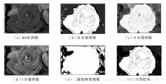
2.3.1 HSI颜色空间中的分割

• HSI颜色空间是面向颜色处理的，用色调H饱和度S描述色彩，用亮度I描述光的强度。
• HSI模型有两个特点：I 分量与图像的彩色信息无关，H 分量和S 分量与人感受颜色的方式是紧密相连的。

from skimage import data, color, io
from matplotlib import pyplot as plt
import numpy as np
import math
import sys


# RGB to HSI
def rgb2hsi(r, g, b):
    r = r / 255
    g = g / 255
    b = b / 255
    num = 0.5 * ((r - g) + (r - b))
    den = ((r - g) * (r - g) + (r - b) * (g - b)) ** 0.5
    if b <= g:
        if den == 0:
            den = sys.float_info.min
        h = math.acos(num / den)
    elif b > g:
        if den == 0:
            den = sys.float_info.min
        h = (2 * math.pi) - math.acos(num / den)
    s = 1 - 3 * min(r, g, b) / (r + g + b)
    i = (r + b + g) / 3
    return int(h), int(s * 100), int(i * 255)


image = io.imread(r'Red-Flower.jpg')
hsi_image = np.zeros(image.shape, dtype='uint8')
for i in range(image.shape[0]):
    for j in range(image.shape[1]):
        r, g, b = image[i, j, :]
        h, s, i = rgb2hsi(r, g, b)
        hsi_image[i, j, :] = (h, s, i)

H = hsi_image[:, :, 0]
S = hsi_image[:, :, 1]
I = hsi_image[:, :, 2]

# 生成二值饱和度模板
S_template = np.zeros(S.shape, dtype='uint8')
for i in range(S.shape[0]):
    for j in range(S.shape[1]):
        if S[i, j] > 0.3 * S.max():
            S_template[i, j] = 1

# 色调图像与二值饱和度模板相乘可得到分割结果
F = np.zeros(H.shape, dtype='uint8')
for i in range(F.shape[0]):
    for j in range(F.shape[1]):
        F[i, j] = H[i, j] * S_template[i, j]

# 显示结果
plt.figure()
plt.axis('off')
plt.imshow(image)  # 显示原始RGB图像

plt.figure()
plt.axis('off')
plt.imshow(H, cmap='gray')  # 显示H分量

plt.figure()
plt.axis('off')
plt.imshow(S, cmap='gray')  # 显示S分量

plt.figure()
plt.axis('off')
plt.imshow(I, cmap='gray')  # 显示I分量

plt.figure()
plt.axis('off')
plt.imshow(S_template, cmap='gray')  # 显示二值饱和度模板

plt.figure()
plt.axis('off')
plt.imshow(F, cmap='gray')  # 显示分割结果

plt.show()

• HSI颜色空间中图像分割的结果
  

2.3.2 RGB颜色空间中的分割

• RGB颜色空间中的分割算法是最直接的，得到的分割效果较好。

from skimage import data, color, io
from matplotlib import pyplot as plt
import numpy as np
import math

image = io.imread(r'Red-Flower.jpg')
r = image[:, :, 0]
g = image[:, :, 1]
b = image[:, :, 2]
# RGB颜色空间中的分割
# 选择样本区域
r_template = r[128:255, 85:169]
# 计算该区域的彩色点的平均向量a的红色分量
r_template_u = np.mean(r_template)
# 计算样本点红色分量的标准差
r_template_d = 0.0
for i in range(r_template.shape[0]):
    for j in range(r_template.shape[1]):
        r_template_d = r_template_d + (r_template[i, j] - r_template_u) * (r_template[i, j] - r_template_u)

r_template_d = math.sqrt(r_template_d / r_template.shape[0] / r_template.shape[1])
# 寻找符合条件的点，r_cut为红色分割图像
r_cut = np.zeros(r.shape, dtype='uint8')
for i in range(r.shape[0]):
    for j in range(r.shape[1]):
        if r[i, j] >= (r_template_u - 1.25 * r_template_d) and r[i, j] <= (r_template_u + 1.25 * r_template_d):
            r_cut[i, j] = 1
# image_cut为根据红色分割后的RGB图像
image_cut = np.zeros(image.shape, dtype='uint8')
for i in range(r.shape[0]):
    for j in range(r.shape[1]):
        if r_cut[i, j] == 1:
            image_cut[i, j, :] = image[i, j, :]

plt.figure()
plt.axis('off')
plt.imshow(image)  # 显示原始图像

plt.figure()
plt.axis('off')
plt.imshow(r)  # 显示R图像

plt.figure()
plt.axis('off')
plt.imshow(g)  # 显示G图像

plt.figure()
plt.axis('off')
plt.imshow(b)  # 显示B图像

plt.figure()
plt.axis('off')
plt.imshow(r_cut)  # 显示红色分割图像图像

plt.figure()
plt.axis('off')
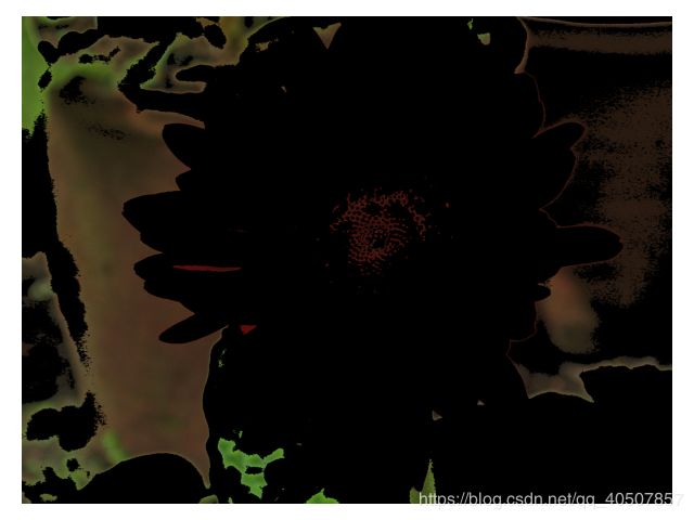
plt.imshow(image_cut)  # 显示分割后的RGB图像

plt.show()

• 与原始RGB图像相比，分割后的RGB图像中绿叶基本被去除，只保留了原始图像中的红色花朵。

• 基于彩色的图像分割主要利用分量图像中感兴趣区域的颜色特征对感兴趣区域进行颜色提取，并弱化背景区域

• 原始RGB图像
  

• R分量图像
  

• G分量图像
  

• B分量图像
  

• 红色分割图像图像
  

• 显示分割后的RGB图像
  

2.4 彩色图像的灰度化

• 灰度图像能以较少的数据表征图像的大部分特征，因此在某些算法的预处理阶段，需要进行彩色图像灰度化，提高后续算法的效率

• 最大值灰度化方法。将彩色图像中像素的R分量、G分量和B分量3个数值的最大值作为灰度图像的灰度值。
  

• 平均灰度化方法。对彩色图像中像素的R分量、G分量和B分量3个数值求平均值作为灰度值。
  

• 加权平均灰度化方法。由于人眼对绿色的敏感度最高，对蓝色的敏感度最低，因此可以根据重要性对三个分量进行加权平均，得到较合理的灰度值。

2.5 小结

• 本章首先对彩色图像进行简要介绍，说明了彩色图像处理的重要意义。
• 讲述了彩色图像的颜色空间，RGB颜色空间和HSI颜色空间以及两种颜色空间的转换。
• 讲述了伪彩色图像处理，重点讨论了强度分层技术和灰度值到彩色图像变换技术。
• 基于彩色的图像分割，主要讨论了基于HSI和RGB的彩色分割。
• 讲述了彩色图像的灰度化，利用最大值灰度化方法、平均值灰度化方法、加权平均值灰度化方法对RGB图像进行灰度化处理。