上面接SSD源码测试
下载源码:
github地址
如果想快速掌握SSD源码请看SS简版代码解读。本人脑子笨,想从易到难慢慢掌握,所以先看了一份简单的代码,再看一份代功能较多的代码对照记忆,这两份代码大体类似,简单版的代码想要训练的话需要改动。
demo_ssd.py
先从demo.py的代码开始吧!!
这里代码就是notebooks/ssd_tests.ipynb里面的代码:
# demo_ssd.py
# encode=utf-8

import os
import math
import random

import numpy as np
import tensorflow as tf
import cv2

slim = tf.contrib.slim
import matplotlib.pyplot as plt
import matplotlib.image as mpimg
import sys
sys.path.append('../')
from nets import ssd_vgg_300, ssd_common, np_methods
from preprocessing import ssd_vgg_preprocessing
from notebooks import visualization
# TensorFlow session: grow memory when needed. TF, DO NOT USE ALL MY GPU MEMORY!!!
gpu_options = tf.GPUOptions(allow_growth=True)
config = tf.ConfigProto(log_device_placement=False, gpu_options=gpu_options)
isess = tf.InteractiveSession(config=config)
# Input placeholder.
net_shape = (300, 300)
data_format = 'NHWC'
img_input = tf.placeholder(tf.uint8, shape=(None, None, 3))
# Evaluation pre-processing: resize to SSD net shape.
image_pre, labels_pre, bboxes_pre, bbox_img = ssd_vgg_preprocessing.preprocess_for_eval(
    img_input, None, None, net_shape, data_format, resize=ssd_vgg_preprocessing.Resize.WARP_RESIZE)
image_4d = tf.expand_dims(image_pre, 0)

# Define the SSD model.
reuse = True if 'ssd_net' in locals() else None
ssd_net = ssd_vgg_300.SSDNet()
with slim.arg_scope(ssd_net.arg_scope(data_format=data_format)):
    predictions, localisations, _, _ = ssd_net.net(image_4d, is_training=False, reuse=reuse)

# Restore SSD model.
ckpt_filename = '../checkpoints/ssd_300_vgg.ckpt'
# ckpt_filename = '../checkpoints/VGG_VOC0712_SSD_300x300_ft_iter_120000.ckpt'
isess.run(tf.global_variables_initializer())
saver = tf.train.Saver()
saver.restore(isess, ckpt_filename)

# SSD default anchor boxes.
ssd_anchors = ssd_net.anchors(net_shape)


# Main image processing routine.
def process_image(img, select_threshold=0.5, nms_threshold=.45, net_shape=(300, 300)):
    # Run SSD network.
    rimg, rpredictions, rlocalisations, rbbox_img = isess.run([image_4d, predictions, localisations, bbox_img],
                                                              feed_dict={img_input: img})

    # Get classes and bboxes from the net outputs.
    rclasses, rscores, rbboxes = np_methods.ssd_bboxes_select(
        rpredictions, rlocalisations, ssd_anchors,
        select_threshold=select_threshold, img_shape=net_shape, num_classes=21, decode=True)

    rbboxes = np_methods.bboxes_clip(rbbox_img, rbboxes)
    rclasses, rscores, rbboxes = np_methods.bboxes_sort(rclasses, rscores, rbboxes, top_k=400)
    rclasses, rscores, rbboxes = np_methods.bboxes_nms(rclasses, rscores, rbboxes, nms_threshold=nms_threshold)
    # Resize bboxes to original image shape. Note: useless for Resize.WARP!
    rbboxes = np_methods.bboxes_resize(rbbox_img, rbboxes)
    return rclasses, rscores, rbboxes
# Test on some demo image and visualize output.
#测试的文件夹
path = '../demo/'
image_names = sorted(os.listdir(path))
#文件夹中的第几张图,-1代表最后一张
img = mpimg.imread(path + image_names[-1])
rclasses, rscores, rbboxes =  process_image(img)

# visualization.bboxes_draw_on_img(img, rclasses, rscores, rbboxes, visualization.colors_plasma)
visualization.plt_bboxes(img, rclasses, rscores, rbboxes)
这里设置了图片的尺寸(300,300),图片的格式为shape='NxHxWxC',对于读取的图片先用preprocess_for_eval进行预处理把图片处理成net_shape的大小,这里留下一个漏洞就是bboxes_pre=[]这个返回值是干什么???,而bbox_img=[0,0,1,1],会慢慢揭晓,流程往下走吧。如下:
net_shape = (300, 300)
data_format = 'NHWC'
img_input = tf.placeholder(tf.uint8, shape=(None, None, 3))
# Evaluation pre-processing: resize to SSD net shape.
image_pre, labels_pre, bboxes_pre, bbox_img = ssd_vgg_preprocessing.preprocess_for_eval(
    img_input, None, None, net_shape, data_format, resize=ssd_vgg_preprocessing.Resize.WARP_RESIZE)
image_4d = tf.expand_dims(image_pre, 0)
构建SSD的模型输出预测的predictions, localisations的占位符。
注意:这里predictions, localisations只是经过初步筛选的预测值,也就是predictions大于某个阀值就保留box和类别预测。这里并没有所谓的NMS等去重手段。
这里的输出localisations.shape = [None, w, h, n_anchors, 4].
predictions.shape=[None, w, h, n_anchors, num_classes].None是batch size.。
ssd_net = ssd_vgg_300.SSDNet()
with slim.arg_scope(ssd_net.arg_scope(data_format=data_format)):
    predictions, localisations, _, _ = ssd_net.net(image_4d, is_training=False, reuse=reuse)
接下来就是套路,拿到ckpt文件中的参数。
# Restore SSD model.
ckpt_filename = '../checkpoints/ssd_300_vgg.ckpt'
# ckpt_filename = '../checkpoints/VGG_VOC0712_SSD_300x300_ft_iter_120000.ckpt'
isess.run(tf.global_variables_initializer())
saver = tf.train.Saver()
saver.restore(isess, ckpt_filename)
接下来就是一件大事了,SSD与Faster R-CNN,YOLO不同就是体现在这里。就是这个 default boxes的设置不同。ssd_anchors 使是设置
# SSD default boxes.
ssd_anchors = ssd_net.anchors(net_shape)
ssd_anchors 是通过anchors设置box的,img_shape=(300,300)
拿到SSD模型上(conv4_3, conv_7) +(conv8_2, conv9_2, conv_10_2, pool_11)所有的default anchor boxes,这里SSD-vgg有8732个。
最后拿到图片的数据,送入SSD网络进行目标检测。
image_names = sorted(os.listdir(path))
#文件夹中的第几张图,-1代表最后一张
img = mpimg.imread(path + image_names[-1])
rclasses, rscores, rbboxes =  process_image(img)
在process_image干什么了??
def process_image(img, select_threshold=0.5, nms_threshold=.45, net_shape=(300, 300)):
    # Run SSD network.
    rimg, rpredictions, rlocalisations, rbbox_img = isess.run([image_4d, predictions, localisations, bbox_img],
                                                              feed_dict={img_input: img})

    # Get classes and bboxes from the net outputs.
    rclasses, rscores, rbboxes = np_methods.ssd_bboxes_select(
        rpredictions, rlocalisations, ssd_anchors,
        select_threshold=select_threshold, img_shape=net_shape, num_classes=21, decode=True)

    rbboxes = np_methods.bboxes_clip(rbbox_img, rbboxes)
    rclasses, rscores, rbboxes = np_methods.bboxes_sort(rclasses, rscores, rbboxes, top_k=400)
    rclasses, rscores, rbboxes = np_methods.bboxes_nms(rclasses, rscores, rbboxes, nms_threshold=nms_threshold)
    # Resize bboxes to original image shape. Note: useless for Resize.WARP!
    rbboxes = np_methods.bboxes_resize(rbbox_img, rbboxes)
    return rclasses, rscores, rbboxes
可以看到rbbox_img 输出值就是[0,0,1,1]。那就是原图的尺寸,而bboxes_pre就是物体的box了,但是test时物体其实是没有的box的所以bboxes_pre的box。
现在可以看到,np_methods就是执行NMS,选择合适的box。
ssd_bboxes_select()函数已经把坐标解码,从[x,y,w, h]解码为[ymin,xmin,ymax,xmax],其中具体的操作慢慢细讲。
rclasses, rscores, rbboxes = np_methods.ssd_bboxes_select(
        rpredictions, rlocalisations, ssd_anchors,
        select_threshold=select_threshold, img_shape=net_shape, num_classes=21, decode=True)
保留前top_k个box
rclasses, rscores, rbboxes = np_methods.bboxes_sort(rclasses, rscores, rbboxes, top_k=400)
保留rscores大于阀值的box
rclasses, rscores, rbboxes = np_methods.bboxes_nms(rclasses, rscores, rbboxes, nms_threshold=nms_threshold)
这里就是把box的大小到原图的尺寸,这里是占原图的比例。
rbboxes = np_methods.bboxes_resize(rbbox_img, rbboxes)
把预测值可视化,这里的坐标已经是原图的比例了,只需要再乘以原尺寸就行了。
visualization.plt_bboxes(img, rclasses, rscores, rbboxes)

demo_test.py的解析大概就到这里了。
下面开始深入探讨。
ssd_vgg_300.py
这里的结构有点混乱,大概只有作者才能理得清
还是老规矩,只看主要结构,在demo.py中出现SSDNet的地方,如下。
# demo.py
略.......
ssd_net = ssd_vgg_300.SSDNet()
with slim.arg_scope(ssd_net.arg_scope(data_format=data_format)):
    predictions, localisations, _, _ = ssd_net.net(image_4d, is_training=False, reuse=reuse)
略.......
ssd_anchors = ssd_net.anchors(net_shape)
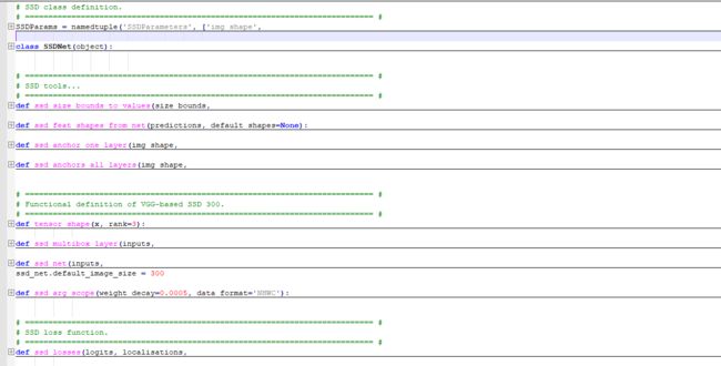
SSDNet()
首先定义ssd需要的参数结构,这里是SSDParams 的参数结构
SSDParams = namedtuple('SSDParameters', ['img_shape',           #输入图像大小
                                         'num_classes',         #分类类别数
                                         'no_annotation_label', #无标注标签
                                         'feat_layers',         #特征层
                                         'feat_shapes',         #特征层形状大小
                                         'anchor_size_bounds',  #锚点框大小上下边界,是与原图相比得到的小数值
                                         'anchor_sizes',        #初始锚点框尺寸
                                         'anchor_ratios',       #锚点框长宽比
                                         'anchor_steps',        #特征图相对原始图像的缩放
                                         'anchor_offset',       #锚点框中心的偏移
                                         'normalizations',      #是否正则化
                                         'prior_scaling'        #是对特征图参考框向gtbox做回归时用到的尺度缩放(0.1,0.1,0.2,0.2)
                                         ])
大体解SSDNet的从体结构:

大体上看SSDNet其实并不复杂从demo.py出发,看看几个主要的函数,如下:
ssd_net = ssd_vgg_300.SSDNet()
with slim.arg_scope(ssd_net.arg_scope(data_format=data_format)):
    predictions, localisations, _, _ = ssd_net.net(image_4d, is_training=False, reuse=reuse)
ssd_anchors = ssd_net.anchors(net_shape)
SSDNet的初始化函数
class SSDNet(object):
    """Implementation of the SSD VGG-based 300 network.

    The default features layers with 300x300 image input are:
      conv4 ==> 38 x 38
      conv7 ==> 19 x 19
      conv8 ==> 10 x 10
      conv9 ==> 5 x 5
      conv10 ==> 3 x 3
      conv11 ==> 1 x 1
    The default image size used to train this network is 300x300.    #训练输入图像尺寸默认为300x300
    """
    default_params = SSDParams(             #默认参数
        img_shape=(300, 300),
        num_classes=21,  #包含背景在内,共21类目标类别
        no_annotation_label=21,
        feat_layers=['block4', 'block7', 'block8', 'block9', 'block10', 'block11'], #特征层名字
        feat_shapes=[(38, 38), (19, 19), (10, 10), (5, 5), (3, 3), (1, 1)],       #特征层尺寸
        anchor_size_bounds=[0.15, 0.90],
        # anchor_size_bounds=[0.20, 0.90],                                        #论文中初始预测框大小为0.2x300~0.9x300;实际代码是[45,270]
        anchor_sizes=[(21., 45.),   #直接给出的每个特征图上起初的锚点框大小;如第一个特征层框大小是h:21;w:45;  共6个特征图用于回归
                      (45., 99.),   #越小的框能够得到原图上更多的局部信息,反之得到更多的全局信息;
                      (99., 153.),
                      (153., 207.),
                      (207., 261.),
                      (261., 315.)],
        # anchor_sizes=[(30., 60.),
        #               (60., 111.),
        #               (111., 162.),
        #               (162., 213.),
        #               (213., 264.),
        #               (264., 315.)],
        anchor_ratios=[[2, .5],             #每个特征层上的每个特征点预测的box长宽比及数量;如:block4: def_boxes:4
                       [2, .5, 3, 1./3],    #block7: def_boxes:6   (ratios中的4个+默认的1:1+额外增加的一个=6)
                       [2, .5, 3, 1./3],    #block8: def_boxes:6
                       [2, .5, 3, 1./3],    #block9: def_boxes:6
                       [2, .5],             #block10: def_boxes:4
                       [2, .5]],            #block11: def_boxes:4   #备注:实际上略去了默认的ratio=1以及多加了一个sqrt(初始框宽*初始框高),后面代码有
        anchor_steps=[8, 16, 32, 64, 100, 300],   #特征图锚点框放大到原始图的缩放比例;
        anchor_offset=0.5,                        #每个锚点框中心点在该特征图cell中心,因此offset=0.5
        normalizations=[20, -1, -1, -1, -1, -1],  #是否归一化,大于0则进行,否则不做归一化;目前看来只对block_4进行正则化,因为该层比较靠前,其norm较大,需做L2正则化(仅仅对每个像素在channel维度做归一化)以保证和后面检测层差异不是很大;
        prior_scaling=[0.1, 0.1, 0.2, 0.2]        #特征图上每个目标与参考框间的尺寸缩放(y,x,h,w)解码时用到
        )

    def __init__(self, params=None):      #网络参数的初始化
        """Init the SSD net with some parameters. Use the default ones
        if none provided.
        """
        if isinstance(params, SSDParams):  #是否有参数输入,是则用输入的,否则使用默认的
            self.params = params           #isinstance是python的內建函数,如果参数1与参数2的类型相同则返回true;
        else:
            self.params = SSDNet.default_params
初始化函数SSDNet的初始化函数功能不多,就是使用默认的初始化参数。简单解释一下参数:
- img_shape=(300, 300) 输入图片的大小
- num_classes=21, 包含背景在内,共21类目标类别
- no_annotation_label=21,
- feat_layers=['block4', 'block7', 'block8', 'block9', 'block10', 'block11'], 特征层名字,ssd_vgg 使用6个特征层进行最后的识别 * feat_shapes=[(38, 38), (19, 19), (10, 10), (5, 5), (3, 3), (1, 1)], 6个特征图的尺寸
- anchor_size_bounds=[0.15, 0.90], 这就是最小最大尺寸,每个box占图片的比例
- anchor_ratios, 每个特征层上的每个特征点预测的box长宽比及数量;
- anchor_steps=[8, 16, 32, 64, 100, 300], 特征图锚点框放大到原始图的缩放比例;
- anchor_offset=0.5 每个锚点框中心点在该特征图cell中心,因此offset=0.5
- normalizations=[20, -1, -1, -1, -1, -1], 是否归一化,大于0则进行,否则不做归一化;目前看来只对block_4进行正则化,因为该层比较靠前,其norm较大,需做L2正则化(仅仅对每个像素在channel维度做归一化)以保证和后面检测层差异不是很大;
- prior_scaling=[0.1, 0.1, 0.2, 0.2] 特征图上每个目标与参考框间的尺寸缩放(y,x,h,w)解码时用到
现在看看SSD的参数空间,因为在test中就是在参数空间运行的
def ssd_arg_scope(weight_decay=0.0005, data_format='NHWC'):  #权重衰减系数=0.0005;其是L2正则化项的系数
    """Defines the VGG arg scope.

    Args:
      weight_decay: The l2 regularization coefficient.

    Returns:
      An arg_scope.
    """
    with slim.arg_scope([slim.conv2d, slim.fully_connected],
                        activation_fn=tf.nn.relu,
                        weights_regularizer=slim.l2_regularizer(weight_decay),
                        weights_initializer=tf.contrib.layers.xavier_initializer(),
                        biases_initializer=tf.zeros_initializer()):
        with slim.arg_scope([slim.conv2d, slim.max_pool2d],
                            padding='SAME',
                            data_format=data_format):
            with slim.arg_scope([custom_layers.pad2d,
                                 custom_layers.l2_normalization,
                                 custom_layers.channel_to_last],
                                data_format=data_format) as sc:
                return sc
这里设值slim.conv2d和slim.fully_connected共有的参数设置,并且slim.conv2d使用SAME的padding方式,设置custom_layers.pad2d层使用custom_layers.l2_normalization方式。
进入SSDNet的net。
def net(self, inputs,                            #定义网络模型,输入图片
            is_training=True,                        #是否训练
            update_feat_shapes=True,                 #是否更新特征层的尺寸
            dropout_keep_prob=0.5,                   #dropout=0.5
            prediction_fn=slim.softmax,              #采用softmax预测结果
            reuse=None,
            scope='ssd_300_vgg'):                    #网络名:ssd_300_vgg   (基础网络时VGG,输入训练图像size是300x300)
        """SSD network definition.
        """
        r = ssd_net(inputs,                               #网络输入参数r
                    num_classes=self.params.num_classes,
                    feat_layers=self.params.feat_layers,
                    anchor_sizes=self.params.anchor_sizes,
                    anchor_ratios=self.params.anchor_ratios,
                    normalizations=self.params.normalizations,
                    is_training=is_training,
                    dropout_keep_prob=dropout_keep_prob,
                    prediction_fn=prediction_fn,
                    reuse=reuse,
                    scope=scope)
        # Update feature shapes (try at least!)    #下面这步我的理解就是让读者自行更改特征层的输入,未必论文中介绍的那几个block
        if update_feat_shapes:                                               #是否更新特征层图像尺寸?
            shapes = ssd_feat_shapes_from_net(r[0], self.params.feat_shapes)  #输入特征层图像尺寸以及inputs(应该是预测的特征尺寸),输出更新后的特征图尺寸列表
            self.params = self.params._replace(feat_shapes=shapes)        #将更新的特征图尺寸shapes替换当前的特征图尺寸
        return r
使用到ssd_net()
那就看看ssd_net()
def ssd_net(inputs,                                             #定义ssd网络结构
            num_classes=SSDNet.default_params.num_classes,      #分类数
            feat_layers=SSDNet.default_params.feat_layers,      #特征层
            anchor_sizes=SSDNet.default_params.anchor_sizes,
            anchor_ratios=SSDNet.default_params.anchor_ratios,
            normalizations=SSDNet.default_params.normalizations, #正则化
            is_training=True,
            dropout_keep_prob=0.5,
            prediction_fn=slim.softmax,
            reuse=None,
            scope='ssd_300_vgg'):
    """SSD net definition.
    """
    # if data_format == 'NCHW':
    #     inputs = tf.transpose(inputs, perm=(0, 3, 1, 2))

    # End_points collect relevant activations for external use.
    end_points = {}   #用于收集每一层输出结果
    with tf.variable_scope(scope, 'ssd_300_vgg', [inputs], reuse=reuse):
        # Original VGG-16 blocks.
        net = slim.repeat(inputs, 2, slim.conv2d, 64, [3, 3], scope='conv1')    #VGG16网络的第一个conv,重复2次卷积,核为3x3,64个特征
        end_points['block1'] = net                                              #conv1_2结果存入end_points,name='block1'
        net = slim.max_pool2d(net, [2, 2], scope='pool1')
        # Block 2.
        net = slim.repeat(net, 2, slim.conv2d, 128, [3, 3], scope='conv2')      #重复2次卷积,核为3x3,128个特征
        end_points['block2'] = net                                              #conv2_2结果存入end_points,name='block2'
        net = slim.max_pool2d(net, [2, 2], scope='pool2')
        # Block 3.
        net = slim.repeat(net, 3, slim.conv2d, 256, [3, 3], scope='conv3')      #重复3次卷积,核为3x3,256个特征
        end_points['block3'] = net                                              #conv3_3结果存入end_points,name='block3'
        net = slim.max_pool2d(net, [2, 2], scope='pool3')
        # Block 4.
        net = slim.repeat(net, 3, slim.conv2d, 512, [3, 3], scope='conv4')       #重复3次卷积,核为3x3,512个特征
        end_points['block4'] = net                                               #conv4_3结果存入end_points,name='block4'
        net = slim.max_pool2d(net, [2, 2], scope='pool4')
        # Block 5.
        net = slim.repeat(net, 3, slim.conv2d, 512, [3, 3], scope='conv5')       #重复3次卷积,核为3x3,512个特征
        end_points['block5'] = net                                               #conv5_3结果存入end_points,name='block5'
        net = slim.max_pool2d(net, [3, 3], stride=1, scope='pool5')

        # Additional SSD blocks.                                                  #去掉了VGG的全连接层
        # Block 6: let's dilate the hell out of it!
        net = slim.conv2d(net, 1024, [3, 3], rate=6, scope='conv6')              #将VGG基础网络最后的池化层结果做扩展卷积(带孔卷积);
        end_points['block6'] = net                                                #conv6结果存入end_points,name='block6'
        net = tf.layers.dropout(net, rate=dropout_keep_prob, training=is_training) #dropout层
        # Block 7: 1x1 conv. Because the fuck.
        net = slim.conv2d(net, 1024, [1, 1], scope='conv7')                          #将dropout后的网络做1x1卷积,输出1024特征,name='block7'
        end_points['block7'] = net
        net = tf.layers.dropout(net, rate=dropout_keep_prob, training=is_training)   #将卷积后的网络继续做dropout

        # Block 8/9/10/11: 1x1 and 3x3 convolutions stride 2 (except lasts).
        end_point = 'block8'
        with tf.variable_scope(end_point):
            net = slim.conv2d(net, 256, [1, 1], scope='conv1x1')           #对上述dropout的网络做1x1卷积,然后做3x3卷积,,输出512特征图,name=‘block8’
            net = custom_layers.pad2d(net, pad=(1, 1))
            net = slim.conv2d(net, 512, [3, 3], stride=2, scope='conv3x3', padding='VALID')
        end_points[end_point] = net
        end_point = 'block9'
        with tf.variable_scope(end_point):
            net = slim.conv2d(net, 128, [1, 1], scope='conv1x1')                 #对上述网络做1x1卷积,然后做3x3卷积,输出256特征图,name=‘block9’
            net = custom_layers.pad2d(net, pad=(1, 1))
            net = slim.conv2d(net, 256, [3, 3], stride=2, scope='conv3x3', padding='VALID')
        end_points[end_point] = net
        end_point = 'block10'
        with tf.variable_scope(end_point):
            net = slim.conv2d(net, 128, [1, 1], scope='conv1x1')               #对上述网络做1x1卷积,然后做3x3卷积,输出256特征图,name=‘block10’
            net = slim.conv2d(net, 256, [3, 3], scope='conv3x3', padding='VALID')
        end_points[end_point] = net
        end_point = 'block11'
        with tf.variable_scope(end_point):
            net = slim.conv2d(net, 128, [1, 1], scope='conv1x1')              #对上述网络做1x1卷积,然后做3x3卷积,输出256特征图,name=‘block11’
            net = slim.conv2d(net, 256, [3, 3], scope='conv3x3', padding='VALID')
        end_points[end_point] = net

        # Prediction and localisations layers. #预测和定位
        predictions = []
        logits = []
        localisations = []
        for i, layer in enumerate(feat_layers):               #遍历特征层
            with tf.variable_scope(layer + '_box'):                #起个命名范围
            p, l = ssd_multibox_layer(end_points[layer],   #做多尺度大小box预测的特征层,返回每个cell中每个先验框预测的类别p和预测的位置l
                                          num_classes,         #种类数
                                          anchor_sizes[i],     #先验框尺度(同一特征图上的先验框尺度和长宽比一致)
                                          anchor_ratios[i],    #先验框长宽比
                                          normalizations[i])   #每个特征正则化信息,目前是只对第一个特征图做归一化操作;
            #把每一层的预测收集
            predictions.append(prediction_fn(p))  #prediction_fn为softmax,预测类别
            logits.append(p) #把每个cell每个先验框预测的类别的概率值存在logits中
            localisations.append(l)   #预测位置信息

        return predictions, localisations, logits, end_points  #返回类别预测结果,位置预测结果,所属某个类别的概率值,以及特征层
ssd_net.default_image_size = 300
SSD网络的主体模型结构比较简单,block1 到 block11都是卷积神经网络,在block8之后开始使用自定义的卷积结构。
在函数的最后使用ssd_multibox_layer对所的feature map构建box和classes预测,在收集的所有的点上进行预测。对于一个wxh的feature map,需要输出的box的shape=[w,h,num_anchors * 4],输出的classes的shape=[w,h,num_anchors * c],这里c=21。
这里的几个返回值:
- predictions: 为softmax之后的预测类别
- logits:把每个cell每个先验框预测的类别的概率值存在logits中
- localisations: 预测位置信息
- end_points 是每个feature map 的输出值。
在网络的后面使用ssd_multibox_layer对网络的feature map进行预测。如下:
def ssd_multibox_layer(inputs,                    #输入特征层
                       num_classes,               #类别数
                       sizes,                     #参考先验框的尺度
                       ratios=[1],                #默认的先验框长宽比为1
                       normalization=-1,          #默认不做正则化
                       bn_normalization=False):
    """Construct a multibox layer, return a class and localization predictions.
    """
    net = inputs
    if normalization > 0:    #如果输入整数,则进行L2正则化
        net = custom_layers.l2_normalization(net, scaling=True)    #对通道所在维度进行正则化,随后乘以gamma缩放系数
    # Number of anchors.
    num_anchors = len(sizes) + len(ratios)  #每层特征图参考先验框的个数[4,6,6,6,4,4]

    # Location.     #每个先验框对应4个坐标信息
    num_loc_pred = num_anchors * 4    #特征图上每个单元预测的坐标所需维度=锚点框数*4
    loc_pred = slim.conv2d(net, num_loc_pred, [3, 3], activation_fn=None,   #通过对特征图进行3x3卷积得到位置信息和类别权重信息
                           scope='conv_loc')                                #该部分是定位信息,输出维度为[特征图h,特征图w,每个单元所有锚点框坐标]
    loc_pred = custom_layers.channel_to_last(loc_pred)
    loc_pred = tf.reshape(loc_pred,                                         #最后整个特征图所有锚点框预测目标位置 tensor为[h*w*每个cell先验框数,4]
                          tensor_shape(loc_pred, 4)[:-1]+[num_anchors, 4])
    # Class prediction.                                                #类别预测
    num_cls_pred = num_anchors * num_classes                            #特征图上每个单元预测的类别所需维度=锚点框数*种类数
    cls_pred = slim.conv2d(net, num_cls_pred, [3, 3], activation_fn=None, #该部分是类别信息,输出维度为[特征图h,特征图w,每个单元所有锚点框对应类别信息]
                           scope='conv_cls')
    cls_pred = custom_layers.channel_to_last(cls_pred)
    cls_pred = tf.reshape(cls_pred,
                          tensor_shape(cls_pred, 4)[:-1]+[num_anchors, num_classes]) #最后整个特征图所有锚点框预测类别 tensor为[h*w*每个cell先验框数,种类数]
    return cls_pred, loc_pred  #返回预测得到的类别和box位置 tensor
这里cls_pred就是网路对feature map的cell的box坐标预测值,loc_pred 就是对cell的box的类别的预测值。
返回到net中
发现网络其实还更新了feature map 的shape,就是防止在SSDParams中设置的feature map的形状与实际输入不符,如果不一致就更新SSDParams 中feat_shapes参数。
如下:
if update_feat_shapes:                                               #是否更新特征层图像尺寸?
            shapes = ssd_feat_shapes_from_net(r[0], self.params.feat_shapes)  #输入特征层图像尺寸以及inputs(应该是预测的特征尺寸),输出更新后的特征图尺寸列表
            self.params = self.params._replace(feat_shapes=shapes)        #将更新的特征图尺寸shapes替换当前的特征图尺寸
ok!!
到这里这行代码其实已经结束了。
# demo.py
predictions, localisations, _, _ = ssd_net.net(image_4d, is_training=False, reuse=reuse)
开始这段:
# demo.py
ssd_anchors = ssd_net.anchors(net_shape)
再次回到SSDNet中,看看anchors
输入原始图像尺寸
返回每个特征层每个参考锚点框的位置及尺寸信息
img_shape = (300, 300)
    def anchors(self, img_shape, dtype=np.float32):             #输入原始图像尺寸;返回每个特征层每个参考锚点框的位置及尺寸信息(x,y,h,w)
        """Compute the default anchor boxes, given an image shape.
        """
        return ssd_anchors_all_layers(img_shape,                #这是个关键函数;检测所有特征层中的参考锚点框位置和尺寸信息
                                      self.params.feat_shapes,
                                      self.params.anchor_sizes,
                                      self.params.anchor_ratios,
                                      self.params.anchor_steps,
                                      self.params.anchor_offset,
                                      dtype)
需要注意是这里的输入参数:
- self.params.feat_shapes= [(38, 38), (19, 19), (10, 10), (5, 5), (3, 3), (1, 1)]
- self.params.anchor_sizes=[0.15, 0.90]
- self.params.anchor_ratios=[[2, .5],[2, .5, 3, 1./3], [2, .5, 3, 1./3],[2, .5, 3, 1./3],[2, .5], [2, .5],
- self.params.anchor_steps=[8, 16, 32, 64, 100, 300]
- self.params.anchor_offset=0.5
跳到ssd_anchors_all_layers()函数
def ssd_anchors_all_layers(img_shape,                 #检测所有特征图中锚点框的四个坐标信息; 输入原始图大小
                           layers_shape,              #每个特征层形状尺寸
                           anchor_sizes,              #起始特征图中框的长宽size
                           anchor_ratios,             #锚点框长宽比列表
                           anchor_steps,              #锚点框相对原图缩放比例
                           offset=0.5,                #锚点中心在每个特征图cell中的偏移
                           dtype=np.float32):
    """Compute anchor boxes for all feature layers.
    """
    layers_anchors = []           #用于存放所有特征图中锚点框位置尺寸信息
    for i, s in enumerate(layers_shape):                 #6个特征图尺寸;如:第0个是38x38
        anchor_bboxes = ssd_anchor_one_layer(img_shape, s,     #分别计算每个特征图中锚点框的位置尺寸信息;
                                             anchor_sizes[i],    #输入:第i个特征图中起始锚点框大小;如第0个是(21., 45.)
                                             anchor_ratios[i],   #输入:第i个特征图中锚点框长宽比列表;如第0个是[2, .5]
                                             anchor_steps[i],    #输入:第i个特征图中锚点框相对原始图的缩放比;如第0个是8
                                             offset=offset, dtype=dtype)  #输入:锚点中心在每个特征图cell中的偏移
        layers_anchors.append(anchor_bboxes)              #将6个特征图中每个特征图上的点对应的锚点框(6个或4个)保存
    return layers_anchors
跳到
def ssd_anchor_one_layer(img_shape,         #检测单个特征图中所有锚点的坐标和尺寸信息(未与原图做除法)
                         feat_shape,
                         sizes,
                         ratios,
                         step,
                         offset=0.5,
                         dtype=np.float32):

    # Compute the position grid: simple way.
    # y, x = np.mgrid[0:feat_shape[0], 0:feat_shape[1]]
    # y = (y.astype(dtype) + offset) / feat_shape[0]
    # x = (x.astype(dtype) + offset) / feat_shape[1]
    # Weird SSD-Caffe computation using steps values...    #归一化到原图的锚点中心坐标(x,y);其坐标值域为(0,1)
    y, x = np.mgrid[0:feat_shape[0], 0:feat_shape[1]]      #对于第一个特征图(block4:38x38);y=[[0,0,……0],[1,1,……1],……[37,37,……,37]];而x=[[0,1,2……,37],[0,1,2……,37],……[0,1,2……,37]]
    y = (y.astype(dtype) + offset) * step / img_shape[0]   #将38个cell对应锚点框的y坐标偏移至每个cell中心,然后乘以相对原图缩放的比例,再除以原图
    x = (x.astype(dtype) + offset) * step / img_shape[1]   #可以得到在原图上,相对原图比例大小的每个锚点中心坐标x,y

    # Expand dims to support easy broadcasting.    #将锚点中心坐标扩大维度
    y = np.expand_dims(y, axis=-1)   #对于第一个特征图,y的shape=38x38x1;x的shape=38x38x1
    x = np.expand_dims(x, axis=-1)

    # Compute relative height and width.
    # Tries to follow the original implementation of SSD for the order.
    num_anchors = len(sizes) + len(ratios)      #该特征图上每个点对应的锚点框数量;如:对于第一个特征图每个点预测4个锚点框(block4:38x38),2+2=4
    h = np.zeros((num_anchors, ), dtype=dtype)     #对于第一个特征图,h的shape=4x;w的shape=4x
    w = np.zeros((num_anchors, ), dtype=dtype)
    # Add first anchor boxes with ratio=1.
    h[0] = sizes[0] / img_shape[0]            #第一个锚点框的高h[0]=起始锚点的高/原图大小的高;例如:h[0]=21/300
    w[0] = sizes[0] / img_shape[1]            #第一个锚点框的宽w[0]=起始锚点的宽/原图大小的宽;例如:h[0]=45/300
    di = 1  #锚点宽个数偏移
    if len(sizes) > 1:
        h[1] = math.sqrt(sizes[0] * sizes[1]) / img_shape[0]    #第二个锚点框的高h[1]=sqrt(起始锚点的高*起始锚点的宽)/原图大小的高;例如:h[1]=sqrt(21*45)/300
        w[1] = math.sqrt(sizes[0] * sizes[1]) / img_shape[1]    #第二个锚点框的高w[1]=sqrt(起始锚点的高*起始锚点的宽)/原图大小的宽;例如:w[1]=sqrt(21*45)/300
        di += 1     #di=2
    for i, r in enumerate(ratios):                            #遍历长宽比例,第一个特征图,r只有两个,2和0.5;共四个锚点宽size(h[0]~h[3])
        h[i+di] = sizes[0] / img_shape[0] / math.sqrt(r)      #例如:对于第一个特征图,h[0+2]=h[2]=21/300/sqrt(2);w[0+2]=w[2]=45/300*sqrt(2)
        w[i+di] = sizes[0] / img_shape[1] * math.sqrt(r)      #例如:对于第一个特征图,h[1+2]=h[3]=21/300/sqrt(0.5);w[1+2]=w[3]=45/300*sqrt(0.5)
    return y, x, h, w
这里解释一下 (y.astype(dtype) + offset) * step,在feature map上认为y是一个像素点的坐标,假如feature map.shape=[38,38].在[[0,0,……0],[1,1,……1],……[37,37,……,37]],因为y是从feature map上取出的所以用的最大坐标为37。那怎么把[37,37]的feature map对应到原图[300,300]呢???
这里的把y=ystep(step=8)就可以把y对应到尺寸为300的图上了。所以这里的的每个点的相当于[300]的8个点。(y+offset) step就是把移到8个点中间。
这里还有一个幺蛾子,就是 anchor_sizes。
anchor_sizes=[(30., 60.),(60., 111.), (111., 162.),(162., 213.),(213., 264.),(264., 315.)]。这里在feature map每个点上需要画出box。在[38,38]的feature map上的box的最小边是30(30是原图的尺寸),反应到[38,38]不多4个格子的大小,同时从这里也可以看出SSD最小的检测只能是38x38个像素的物体。
h[0] = sizes[0] / img_shape[0]就是把在原图上box归一化到[0,1]。
来张图解释:
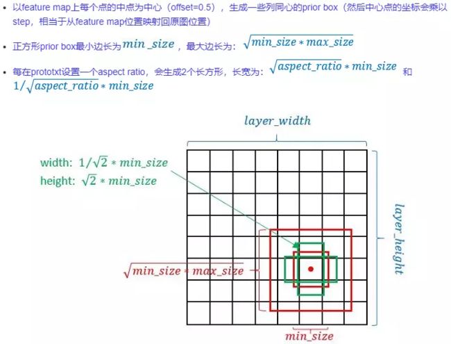
所有的box的尺寸:
sizes:  (21.0, 45.0)
h, w:  [[0.07       0.10246951 0.04949747 0.09899495]
 [0.07       0.10246951 0.09899495 0.04949747]]
sizes:  (45.0, 99.0)
h, w:  [[0.15       0.22248596 0.10606602 0.21213204 0.08660254 0.25980762]
 [0.15       0.22248596 0.21213204 0.10606602 0.25980762 0.08660254]]
sizes:  (99.0, 153.0)
h, w:  [[0.33       0.41024384 0.23334524 0.46669048 0.19052559 0.5715768 ]
 [0.33       0.41024384 0.46669048 0.23334524 0.5715768  0.19052559]]
sizes:  (153.0, 207.0)
h, w:  [[0.51       0.5932116  0.36062446 0.7212489  0.29444864 0.8833459 ]
 [0.51       0.5932116  0.7212489  0.36062446 0.8833459  0.29444864]]
sizes:  (207.0, 261.0)
h, w:  [[0.69       0.7747903  0.48790368 0.97580737]
 [0.69       0.7747903  0.97580737 0.48790368]]
sizes:  (261.0, 315.0)
h, w:  [[0.87      0.9557719 0.6151829 1.2303658]
 [0.87      0.9557719 1.2303658 0.6151829]]
每个feature map上cell的box的坐标基于ssd输出得到的,是固定尺寸。
现在所有的anchors box也得到了,回到demo.py中吧。
开始进行非极大值抑制np_methods,
这里竟然是在numpy里面执行的。
这里先抽取特征。
rclasses, rscores, rbboxes = np_methods.ssd_bboxes_select(
        rpredictions, rlocalisations, ssd_anchors,
        select_threshold=select_threshold, img_shape=net_shape, num_classes=21, decode=True)
跳到ssd_bboxes_select()抽取box坐标所对应的feature map。
def ssd_bboxes_select(predictions_net,
                      localizations_net,
                      anchors_net,
                      select_threshold=0.5,
                      img_shape=(300, 300),
                      num_classes=21,
                      decode=True):
    """Extract classes, scores and bounding boxes from network output layers.

    Return:
      classes, scores, bboxes: Numpy arrays...
    """
    l_classes = []
    l_scores = []
    l_bboxes = []
    # l_layers = []
    # l_idxes = []
    for i in range(len(predictions_net)):
        classes, scores, bboxes = ssd_bboxes_select_layer(
            predictions_net[i], localizations_net[i], anchors_net[i],
            select_threshold, img_shape, num_classes, decode)
        l_classes.append(classes)
        l_scores.append(scores)
        l_bboxes.append(bboxes)
        # Debug information.
        # l_layers.append(i)
        # l_idxes.append((i, idxes))

    classes = np.concatenate(l_classes, 0)
    scores = np.concatenate(l_scores, 0)
    bboxes = np.concatenate(l_bboxes, 0)
    return classes, scores, bboxes
极大值预测之前需要把box对应的值从feature map中抽取出来,使用
ssd_bboxes_select_layer()
def ssd_bboxes_select_layer(predictions_layer,
                            localizations_layer,
                            anchors_layer,
                            select_threshold=0.5,
                            img_shape=(300, 300),
                            num_classes=21,
                            decode=True):
    """Extract classes, scores and bounding boxes from features in one layer.

    Return:
      classes, scores, bboxes: Numpy arrays...
    """
    # First decode localizations features if necessary.
    if decode:
        localizations_layer = ssd_bboxes_decode(localizations_layer, anchors_layer)

    # Reshape features to: Batches x N x N_labels | 4.
    p_shape = predictions_layer.shape
    batch_size = p_shape[0] if len(p_shape) == 5 else 1
    predictions_layer = np.reshape(predictions_layer,
                                   (batch_size, -1, p_shape[-1]))
    l_shape = localizations_layer.shape
    localizations_layer = np.reshape(localizations_layer,
                                     (batch_size, -1, l_shape[-1]))

    # Boxes selection: use threshold or score > no-label criteria.
    if select_threshold is None or select_threshold == 0:
        # Class prediction and scores: assign 0. to 0-class
        classes = np.argmax(predictions_layer, axis=2)
        scores = np.amax(predictions_layer, axis=2)
        mask = (classes > 0)
        classes = classes[mask]
        scores = scores[mask]
        bboxes = localizations_layer[mask]
    else:
        sub_predictions = predictions_layer[:, :, 1:]
        idxes = np.where(sub_predictions > select_threshold)
        classes = idxes[-1]+1
        scores = sub_predictions[idxes]
        bboxes = localizations_layer[idxes[:-1]]

    return classes, scores, bboxes
解码box所对应的坐标
def ssd_bboxes_decode(feat_localizations,
                      anchor_bboxes,
                      prior_scaling=[0.1, 0.1, 0.2, 0.2]):
    """Compute the relative bounding boxes from the layer features and
    reference anchor bounding boxes.

    Return:
      numpy array Nx4: ymin, xmin, ymax, xmax
    """
    # Reshape for easier broadcasting.
    l_shape = feat_localizations.shape
    feat_localizations = np.reshape(feat_localizations,
                                    (-1, l_shape[-2], l_shape[-1]))
    yref, xref, href, wref = anchor_bboxes
    xref = np.reshape(xref, [-1, 1])
    yref = np.reshape(yref, [-1, 1])

    # Compute center, height and width
    cx = feat_localizations[:, :, 0] * wref * prior_scaling[0] + xref
    cy = feat_localizations[:, :, 1] * href * prior_scaling[1] + yref
    w = wref * np.exp(feat_localizations[:, :, 2] * prior_scaling[2])
    h = href * np.exp(feat_localizations[:, :, 3] * prior_scaling[3])
    # bboxes: ymin, xmin, xmax, ymax.
    bboxes = np.zeros_like(feat_localizations)
    bboxes[:, :, 0] = cy - h / 2.
    bboxes[:, :, 1] = cx - w / 2.
    bboxes[:, :, 2] = cy + h / 2.
    bboxes[:, :, 3] = cx + w / 2.
    # Back to original shape.
    bboxes = np.reshape(bboxes, l_shape)
    return bboxes
解释一下输入的参数
feat_localizations=这是网路的box的预测坐标[]
anchor_bboxes=这里feature map的default anchor boxes坐标[]
参考:
深刻解读SSD tensorflow及源码详解
SSD关键源码解析
目标检测|SSD原理与实现
SSD-Tensorflow超详细解析【一】:加载模型对图片进行测试