笔记:动手学深度学习pytorch(文本预处理,语言模型与数据集,循环神经网络)
- 文本预处理
- 文本
文本是一类序列数据,一篇文章可以看作是字符或单词的序列
- 处理步骤
- 读入文本
- 分词
- 建立字典,将每个词映射到一个唯一的索引(index)
- 将文本从词的序列转换为索引的序列,方便输入模型
- 读入文本
这里用一部英文小说,即H. G. Well的Time Machine,作为示例,展示文本预处理的具体过程。
import collections
import re
def read_time_machine():
    with open('/home/kesci/input/timemachine7163/timemachine.txt', 'r') as f:
        lines = [re.sub('[^a-z]+', ' ', line.strip().lower()) for line in f]
    return lines
lines = read_time_machine()
print('# sentences %d' % len(lines))
这里会返回有多少个行
- 分词
我们将一个句子分为若干个词(token),转换为一个词的序列
def tokenize(sentences, token='word'):
    """Split sentences into word or char tokens"""
    if token == 'word':
        return [sentence.split(' ') for sentence in sentences]
    elif token == 'char':
        return [list(sentence) for sentence in sentences]
    else:
        print('ERROR: unkown token type '+token)
tokens = tokenize(lines
)
tokens[0:2]
![]()
但是这种分词方法有一个问题
- 标点符号通常可以提供语义信息,但是在这种分词方法将其丢弃了
- 建立字典
为了便于处理模型,字符的可处理性并没有数字好,所以我们需要先构建一个字典(vocabulary),将每个词映射到一个唯一的索引编号。
class Vocab(object):
    def __init__(self, tokens, min_freq=0, use_special_tokens=False):
        counter = count_corpus(tokens)  # :
        self.token_freqs = list(counter.items())
        self.idx_to_token = []
        if use_special_tokens:
            # padding, begin of sentence, end of sentence, unknown
            self.pad, self.bos, self.eos, self.unk = (0, 1, 2, 3)
            self.idx_to_token += ['', '', '', '']
        else:
            self.unk = 0
            self.idx_to_token += ['']
        self.idx_to_token += [token for token, freq in self.token_freqs
                        if freq >= min_freq and token not in self.idx_to_token]
        self.token_to_idx = dict()
        for idx, token in enumerate(self.idx_to_token):
            self.token_to_idx[token] = idx
    def __len__(self):
        return len(self.idx_to_token)
    def __getitem__(self, tokens):
        if not isinstance(tokens, (list, tuple)):
            return self.token_to_idx.get(tokens, self.unk)
        return [self.__getitem__(token) for token in tokens]
    def to_tokens(self, indices):
        if not isinstance(indices, (list, tuple)):
            return self.idx_to_token[indices]
        return [self.idx_to_token[index] for index in indices]
def count_corpus(sentences):
    tokens = [tk for st in sentences for tk in st]
    return collections.Counter(tokens)  # 返回一个字典,记录每个词的出现次数
- 将词转换为索引
我们通过建立的字典,我们可以将原文本中的句子从单词序列转换为索引序列
or i in range(8, 10):
    print('words:', tokens[i])
    print('indices:', vocab[tokens[i]])

- 语言模型与数据集
- 语言模型
一段自然语言文本可以看作是一个离散时间序列,给定一个长度为 T \boldsymbol{T} T的词的序列 w 1 , w 2 , … , w T w_1, w_2, \ldots, w_T w1,w2,…,wT,语言模型的目标就是评估该序列是否合理,即计算该序列的概率:
P ( w 1 , w 2 , … , w T ) . P(w_1, w_2, \ldots, w_T). P(w1,w2,…,wT).
假设序列 w 1 , w 2 , … , w T w_1, w_2, \ldots, w_T w1,w2,…,wT中的每个词是依次生成的,我们有
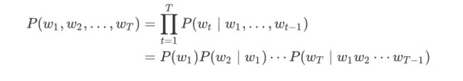
例如,一段含有4个词的文本序列的概率
P ( w 1 , w 2 , w 3 , w 4 ) = P ( w 1 ) P ( w 2 ∣ w 1 ) P ( w 3 ∣ w 1 , w 2 ) P ( w 4 ∣ w 1 , w 2 , w 3 ) . P(w_1, w_2, w_3, w_4) = P(w_1) P(w_2 \mid w_1) P(w_3 \mid w_1, w_2) P(w_4 \mid w_1, w_2, w_3). P(w1,w2,w3,w4)=P(w1)P(w2∣w1)P(w3∣w1,w2)P(w4∣w1,w2,w3).
语言模型的参数就是词的概率以及给定前几个词情况下的条件概率。设训练数据集为一个大型文本语料库,如维基百科的所有条目,词的概率可以通过该词在训练数据集中的相对词频来计算,例如, w 1 \boldsymbol{w_1} w1的概率可以计算为:
P ^ ( w 1 ) = n ( w 1 ) n \hat P(w_1) = \frac{n(w_1)}{n} P^(w1)=nn(w1)
类似的,给定 w 1 \boldsymbol{w_1} w1情况下, w 2 \boldsymbol{w_2} w2的条件概率可以计算为:
P ^ ( w 2 ∣ w 1 ) = n ( w 1 , w 2 ) n ( w 1 ) \hat P(w_2 \mid w_1) = \frac{n(w_1, w_2)}{n(w_1)} P^(w2∣w1)=n(w1)n(w1,w2)
- n元语法
序列长度增加,计算和存储多个词共同出现的概率的复杂度会呈指数级增加。 n n n元语法通过马尔可夫假设简化模型,马尔科夫假设是指一个词的出现只与前面 n n n个词相关,即 n n n阶马尔可夫链(Markov chain of order n n n),如果 n = 1 n=1 n=1,那么有 P ( w 3 ∣ w 1 , w 2 ) = P ( w 3 ∣ w 2 ) P(w_3 \mid w_1, w_2) = P(w_3 \mid w_2) P(w3∣w1,w2)=P(w3∣w2)。基于 n − 1 n-1 n−1阶马尔可夫链,我们可以将语言模型改写为
P ( w 1 , w 2 , … , w T ) = ∏ t = 1 T P ( w t ∣ w t − ( n − 1 ) , … , w t − 1 ) . P(w_1, w_2, \ldots, w_T) = \prod_{t=1}^T P(w_t \mid w_{t-(n-1)}, \ldots, w_{t-1}) . P(w1,w2,…,wT)=∏t=1TP(wt∣wt−(n−1),…,wt−1).
长度为4的序列 w 1 , w 2 , w 3 , w 4 w_1, w_2, w_3, w_4 w1,w2,w3,w4在一元语法、二元语法和三元语法中的概率分别为
P ( w 1 , w 2 , w 3 , w 4 ) P(w_1, w_2, w_3, w_4) P(w1,w2,w3,w4) = P ( w 1 ) P(w_1) P(w1) P ( w 2 ) P(w_2) P(w2) P ( w 3 ) P(w_3) P(w3) P ( w 4 ) P(w_4) P(w4)
P ( w 1 , w 2 , w 3 , w 4 ) P(w_1, w_2, w_3, w_4) P(w1,w2,w3,w4) = P ( w 1 ) P(w_1) P(w1) P ( w 2 ∣ w 1 ) P(w_2 \mid w_1) P(w2∣w1) P ( w 3 ∣ w 2 ) P(w_3\mid w_2) P(w3∣w2) P ( w 4 ∣ w 3 ) P(w_4 \mid w_3) P(w4∣w3)
P ( w 1 , w 2 , w 3 , w 4 ) P(w_1, w_2, w_3, w_4) P(w1,w2,w3,w4) = P ( w 1 ) P(w_1) P(w1) P ( w 2 ∣ w 1 ) P(w_2 \mid w_1) P(w2∣w1) P ( w 3 ∣ w 1 , w 2 ) P(w_3 \mid w_1, w_2) P(w3∣w1,w2) P ( w 4 ∣ w 2 , w 3 ) P(w_4 \mid w_2, w_3) P(w4∣w2,w3)
但是 n n n元语法有两个缺陷
- 参数空间过大
- 数据稀疏
- 语言模型数据集
- 读取数据集
with open('/home/kesci/input/jaychou_lyrics4703/jaychou_lyrics.txt') as f:
corpus_chars = f.read()
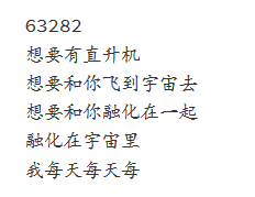
print(len(corpus_chars))
print(corpus_chars[: 40])
corpus_chars = corpus_chars.replace('\n', ' ').replace('\r', ' ')
corpus_chars = corpus_chars[: 10000]
- 建立字符索引
idx_to_char = list(set(corpus_chars)) # 去重,得到索引到字符的映射
char_to_idx = {char: i for i, char in enumerate(idx_to_char)} # 字符到索引的映射
vocab_size = len(char_to_idx)
print(vocab_size)
corpus_indices = [char_to_idx[char] for char in corpus_chars]  # 将每个字符转化为索引,得到一个索引的序列
sample = corpus_indices[: 20]
print('chars:', ''.join([idx_to_char[idx] for idx in sample]))
print('indices:', sample)

- 时序数据采样
在训练中我们需要每次随机读取小批量样本和标签。与之前章节的实验数据不同的是,时序数据的一个样本通常包含连续的字符。假设时间步数为5,样本序列为5个字符,即“想”“要”“有”“直”“升”。该样本的标签序列为这些字符分别在训练集中的下一个字符,即“要”“有”“直”“升”“机”,即 X X X=“想要有直升”, Y Y Y=“要有直升机”。
如果序列的长度为 T T T,时间步数为 n n n,那么一共有 T − n T-n T−n个合法的样本,但是这些样本有大量的重合,我们通常采用更加高效的采样方式。我们有两种方式对时序数据进行采样,分别是随机采样和相邻采样。
- 随机采样
下面的代码每次从数据里随机采样一个小批量。其中批量大小batch_size是每个小批量的样本数,num_steps是每个样本所包含的时间步数。 在随机采样中,每个样本是原始序列上任意截取的一段序列,相邻的两个随机小批量在原始序列上的位置不一定相毗邻。
import torch
import random
def data_iter_random(corpus_indices, batch_size, num_steps, device=None):
    # 减1是因为对于长度为n的序列,X最多只有包含其中的前n - 1个字符
    num_examples = (len(corpus_indices) - 1) // num_steps  # 下取整,得到不重叠情况下的样本个数
    example_indices = [i * num_steps for i in range(num_examples)]  # 每个样本的第一个字符在corpus_indices中的下标
    random.shuffle(example_indices)
    def _data(i):
        # 返回从i开始的长为num_steps的序列
        return corpus_indices[i: i + num_steps]
    if device is None:
        device = torch.device('cuda' if torch.cuda.is_available() else 'cpu')
    for i in range(0, num_examples, batch_size):
        # 每次选出batch_size个随机样本
        batch_indices = example_indices[i: i + batch_size]  # 当前batch的各个样本的首字符的下标
        X = [_data(j) for j in batch_indices]
        Y = [_data(j + 1) for j in batch_indices]
        yield torch.tensor(X, device=device), torch.tensor(Y, device=device)
函数测试
my_seq = list(range(30))
for X, Y in data_iter_random(my_seq, batch_size=2, num_steps=6):
    print('X: ', X, '\nY:', Y, '\n')

- 相邻采样
在相邻采样中,相邻的两个随机小批量在原始序列上的位置相毗邻。
def data_iter_consecutive(corpus_indices, batch_size, num_steps, device=None):
    if device is None:
        device = torch.device('cuda' if torch.cuda.is_available() else 'cpu')
    corpus_len = len(corpus_indices) // batch_size * batch_size  # 保留下来的序列的长度
    corpus_indices = corpus_indices[: corpus_len]  # 仅保留前corpus_len个字符
    indices = torch.tensor(corpus_indices, device=device)
    indices = indices.view(batch_size, -1)  # resize成(batch_size, )
    batch_num = (indices.shape[1] - 1) // num_steps
    for i in range(batch_num):
        i = i * num_steps
        X = indices[:, i: i + num_steps]
        Y = indices[:, i + 1: i + num_steps + 1]
        yield X, Y
for X, Y in data_iter_consecutive(my_seq, batch_size=2, num_steps=6):
    print('X: ', X, '\nY:', Y, '\n')

- 循环神经网络

由图上的内容可以很好看出我们是基于当前的输入序列和过去的输入序列来预测序列的下一个字符
循环神经网络引入一个隐藏变量 H H H,用 H t H_t Ht表示 H H H在时间步 t t t的值。 H — t H—_t H—t的计算基于 X t X_t Xt和 H t − 1 H_{t-1} Ht−1,可以认为 H t H_t Ht记录了到当前字符为止的序列信息,利用 H t H_t Ht对序列的下一个字符进行预测。
- 构造
我们先看循环神经网络的具体构造。假设 X t ∈ R n × d \boldsymbol{X}_t \in \mathbb{R}^{n \times d} Xt∈Rn×d是时间步的小批量输入, H t ∈ R n × h \boldsymbol{H}_t \in \mathbb{R}^{n \times h} Ht∈Rn×h是该时间步的隐藏变量,则:
H t = ϕ ( X t W x h + H t − 1 W h h + b h ) . \boldsymbol{H}_t = \phi(\boldsymbol{X}_t \boldsymbol{W}_{xh} + \boldsymbol{H}_{t-1} \boldsymbol{W}_{hh} + \boldsymbol{b}_h). Ht=ϕ(XtWxh+Ht−1Whh+bh).
在时间步 t t t,输出层的输出为:
O t = H t W h q + b q . \boldsymbol{O}_t = \boldsymbol{H}_t \boldsymbol{W}_{hq} + \boldsymbol{b}_q. Ot=HtWhq+bq.
- one-hot向量
def one_hot(x, n_class, dtype=torch.float32):
    result = torch.zeros(x.shape[0], n_class, dtype=dtype, device=x.device)  # shape: (n, n_class)
    result.scatter_(1, x.long().view(-1, 1), 1)  # result[i, x[i, 0]] = 1
    return result
x = torch.tensor([0, 2])
x_one_hot = one_hot(x, vocab_size)
print(x_one_hot)
print(x_one_hot.shape)
print(x_one_hot.sum(axis=1))

one-hot向量的作用可以理解为一个数组,这个数组的第 i i i个位置是1,代表了这个字符的位置,其他位置全部为0
- 裁剪梯度
循环神经网络中较容易出现梯度衰减或梯度爆炸,这会导致网络几乎无法训练。裁剪梯度(clip gradient)是一种应对梯度爆炸的方法。假设我们把所有模型参数的梯度拼接成一个向量 g g g,并设裁剪的阈值是 θ \theta θ。裁剪后的 L 2 L_2 L2梯度的范数不超过 θ \theta θ。
min ( θ ∥ g ∥ , 1 ) g \min\left(\frac{\theta}{\|\boldsymbol{g}\|}, 1\right)\boldsymbol{g} min(∥g∥θ,1)g
def grad_clipping(params, theta, device):
    norm = torch.tensor([0.0], device=device)
    for param in params:
        norm += (param.grad.data ** 2).sum()
    norm = norm.sqrt().item()
    if norm > theta:
        for param in params:
            param.grad.data *= (theta / norm)
- 困惑度
困惑度是用来评价语言模型的好坏的
- 最佳情况下,模型总是把标签类别的概率预测为1,此时困惑度为1;
- 最坏情况下,模型总是把标签类别的概率预测为0,此时困惑度为正无穷;
- 基线情况下,模型总是预测所有类别的概率都相同,此时困惑度为类别个数。
- 循环神经网络简介实现
我们使用Pytorch中的nn.RNN来构造循环神经网络。
input_size - The number of expected features in the input x
hidden_size – The number of features in the hidden state h
nonlinearity – The non-linearity to use. Can be either 'tanh' or 'relu'. Default: 'tanh'
batch_first – If True, then the input and output tensors are provided as (batch_size, num_steps, input_size). Default: False
这里的batch_first决定了输入的形状,我们使用默认的参数False,对应的输入形状是 (num_steps, batch_size, input_size)。
forward函数的参数为:
input of shape (num_steps, batch_size, input_size): tensor containing the features of the input sequence.
h_0 of shape (num_layers * num_directions, batch_size, hidden_size): tensor containing the initial hidden state for each element in the batch. Defaults to zero if not provided. If the RNN is bidirectional, num_directions should be 2, else it should be 1.
forward函数的返回值是:
output of shape (num_steps, batch_size, num_directions * hidden_size): tensor containing the output features (h_t) from the last layer of the RNN, for each t.
h_n of shape (num_layers * num_directions, batch_size, hidden_size): tensor containing the hidden state for t = num_steps.