python计算机视觉作业1

开始学python计算机视觉这本教材，博主写这篇博文记录下本书第一章的部分例程
1、图像轮廓和直方图
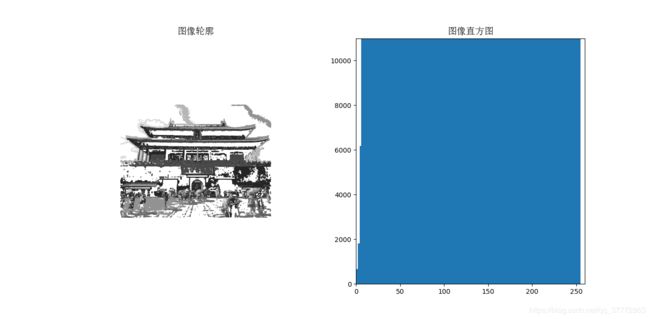
下面我们看两个特别的例子：图像轮廓线和图线等高线。在画图像轮廓前需要转换为灰度图像，因为轮廓需要获取每个坐标[x, y]位置的像素值。下面是画图像轮廓和直方图的代码：

 # -*- coding: utf-8 -*-
from PIL import Image
from pylab import *

# 添加中文字体支持
from matplotlib.font_manager import FontProperties
font = FontProperties(fname=r"c:\windows\fonts\SimSun.ttc", size=14)
im = array(Image.open('../data/empire.jpg').convert('L'))  # 打开图像，并转成灰度图像

figure()
subplot(121)
gray()
contour(im, origin='image')
axis('equal')
axis('off')
title(u'图像轮廓', fontproperties=font)

subplot(122)
hist(im.flatten(), 128)
title(u'图像直方图', fontproperties=font)
plt.xlim([0,260])
plt.ylim([0,11000])

show()

运行结果：

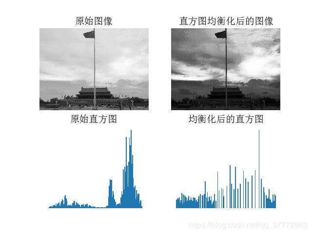
2、直方图均衡化
一个及其有用的例子是灰度变换后进行直方图均衡化。图像均衡化作为预处理操作，在归一化图像强度时是一个很好的方式，并且通过直方图均衡化可以增加图像对比度。下面是对图像进行均衡化处理的例子：

 # -*- coding: utf-8 -*-
from PIL import Image
from pylab import *
from PCV.tools import imtools

# 添加中文字体支持
from matplotlib.font_manager import FontProperties
font = FontProperties(fname=r"c:\windows\fonts\SimSun.ttc", size=14)

im = array(Image.open('../data/empire.jpg').convert('L'))  # 打开图像，并转成灰度图像
#im = array(Image.open('../data/AquaTermi_lowcontrast.JPG').convert('L'))
im2, cdf = imtools.histeq(im)

figure()
subplot(2, 2, 1)
axis('off')
gray()
title(u'原始图像', fontproperties=font)
imshow(im)

subplot(2, 2, 2)
axis('off')
title(u'直方图均衡化后的图像', fontproperties=font)
imshow(im2)

subplot(2, 2, 3)
axis('off')
title(u'原始直方图', fontproperties=font)
#hist(im.flatten(), 128, cumulative=True, normed=True)
hist(im.flatten(), 128, normed=True)

subplot(2, 2, 4)
axis('off')
title(u'均衡化后的直方图', fontproperties=font)
#hist(im2.flatten(), 128, cumulative=True, normed=True)
hist(im2.flatten(), 128, normed=True)

show()

运行上面代码，可以得到书中的结果：

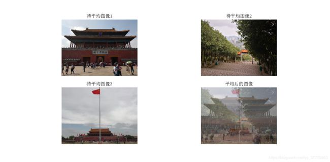
3、图像平均
对图像取平均是一种图像降噪的简单方法，经常用于产生艺术效果。假设所有的图像具有相同的尺寸，我们可以对图像相同位置的像素加取平均，下面是一个演示对图像取平均的例子：

# -*- coding: utf-8 -*-
from PCV.tools.imtools import get_imlist
from PIL import Image
from pylab import *
from PCV.tools import imtools

# 添加中文字体支持
from matplotlib.font_manager import FontProperties
font = FontProperties(fname=r"c:\windows\fonts\SimSun.ttc", size=14)

filelist = get_imlist('../data/avg/') #获取convert_images_format_test文件夹下的图片文件名(包括后缀名)
avg = imtools.compute_average(filelist)

for impath in filelist:
        im1 = array(Image.open(impath))
        subplot(2, 2, filelist.index(impath)+1)
        imshow(im1)
        imNum=str(filelist.index(impath)+1)
        title(u'待平均图像'+imNum, fontproperties=font)
        axis('off')
subplot(2, 2, 4)
imshow(avg)
title(u'平均后的图像', fontproperties=font)
axis('off')

show()

运行上面代码，可得对三幅图像平均后的效果，如下图：

4、SciPy模块
SciPy是一个开源的数学工具包，它是建立在NumPy的基础上的。它提供了很多有效的常规操作，包括数值综合、最优化、统计、信号处理以及图像处理。正如接下来所展示的，SciPy库包含了很多有用的模块。SciPy库可以再[http://scipy.org/Download]下载。
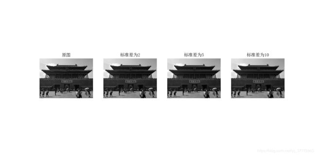
4.1图像模糊
一个经典的并且十分有用的图像卷积例子是对图像进行高斯模糊。高斯模糊可以用于定义图像尺度、计算兴趣点以及很多其他的应用场合。下面是对图像进行模糊显示原书P017 Fig1-9的例子。

 # -*- coding: utf-8 -*-
from PIL import Image
from pylab import *
from scipy.ndimage import filters

# 添加中文字体支持
from matplotlib.font_manager import FontProperties
font = FontProperties(fname=r"c:\windows\fonts\SimSun.ttc", size=14)

#im = array(Image.open('board.jpeg'))
im = array(Image.open('../data/empire.jpg').convert('L'))

figure()
gray()
axis('off')
subplot(1, 4, 1)
axis('off')
title(u'原图', fontproperties=font)
imshow(im)

for bi, blur in enumerate([2, 5, 10]):
  im2 = zeros(im.shape)
  im2 = filters.gaussian_filter(im, blur)
  im2 = np.uint8(im2)
  imNum=str(blur)
  subplot(1, 4, 2 + bi)
  axis('off')
  title(u'标准差为'+imNum, fontproperties=font)
  imshow(im2)

#如果是彩色图像，则分别对三个通道进行模糊
#for bi, blur in enumerate([2, 5, 10]):
#  im2 = zeros(im.shape)
#  for i in range(3):
#    im2[:, :, i] = filters.gaussian_filter(im[:, :, i], blur)
#  im2 = np.uint8(im2)
#  subplot(1, 4,  2 + bi)
#  axis('off')
#  imshow(im2)

show()

运行结果，第一幅图为待模糊图像，第二幅用高斯标准差为2进行模糊，第三幅用高斯标准差为5进行模糊，最后一幅用高斯标准差为10进行模糊。关于该模块的使用以及参数选择的更多细节，可以参阅SciPy scipy.ndimage文档[docs.scipy.org/doc/scipy/reference/ndimage.html]。

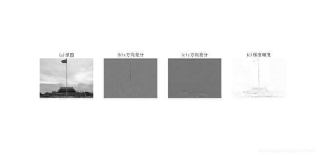
5、图像差分
图像强度的改变是一个重要的信息，被广泛用以很多应用中

# -*- coding: utf-8 -*-
from PIL import Image
from pylab import *
from scipy.ndimage import filters
import numpy

# 添加中文字体支持
from matplotlib.font_manager import FontProperties
font = FontProperties(fname=r"c:\windows\fonts\SimSun.ttc", size=14)

im = array(Image.open('../data/empire.jpg').convert('L'))
gray()

subplot(1, 4, 1)
axis('off')
title(u'(a)原图', fontproperties=font)
imshow(im)

# Sobel derivative filters
imx = zeros(im.shape)
filters.sobel(im, 1, imx)
subplot(1, 4, 2)
axis('off')
title(u'(b)x方向差分', fontproperties=font)
imshow(imx)

imy = zeros(im.shape)
filters.sobel(im, 0, imy)
subplot(1, 4, 3)
axis('off')
title(u'(c)y方向差分', fontproperties=font)
imshow(imy)

#mag = numpy.sqrt(imx**2 + imy**2)
mag = 255-numpy.sqrt(imx**2 + imy**2)
subplot(1, 4, 4)
title(u'(d)梯度幅度', fontproperties=font)
axis('off')
imshow(mag)

show()

运行上面代码，可得如下的运行结果：
第一幅图为待模糊图像，第二幅用高斯标准差为2进行模糊，第三幅用高斯标准差为5进行模糊，最后一幅用高斯标准差为10进行模糊。关于该模块的使用以及参数选择的更多细节，可以参阅SciPy scipy.ndimage文档[docs.scipy.org/doc/scipy/reference/ndimage.html]。

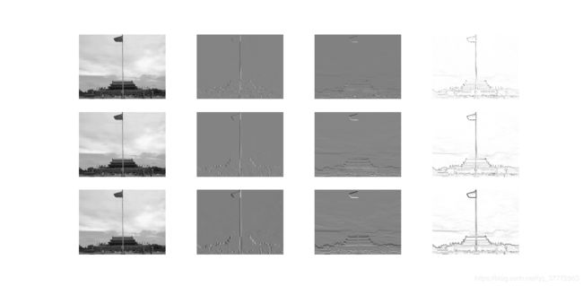
下面再看一个高斯差分的例子

 # -*- coding: utf-8 -*-
from PIL import Image
from pylab import *
from scipy.ndimage import filters
import numpy

# 添加中文字体支持
#from matplotlib.font_manager import FontProperties
#font = FontProperties(fname=r"c:\windows\fonts\SimSun.ttc", size=14)

def imx(im, sigma):
    imgx = zeros(im.shape)
    filters.gaussian_filter(im, sigma, (0, 1), imgx)
    return imgx


def imy(im, sigma):
    imgy = zeros(im.shape)
    filters.gaussian_filter(im, sigma, (1, 0), imgy)
    return imgy


def mag(im, sigma):
    # there's also gaussian_gradient_magnitude()
    #mag = numpy.sqrt(imgx**2 + imgy**2)
    imgmag = 255 - numpy.sqrt(imgx ** 2 + imgy ** 2)
    return imgmag


im = array(Image.open('../data/empire.jpg').convert('L'))
figure()
gray()

sigma = [2, 5, 10]

for i in  sigma:
    subplot(3, 4, 4*(sigma.index(i))+1)
    axis('off')
    imshow(im)
    imgx=imx(im, i)
    subplot(3, 4, 4*(sigma.index(i))+2)
    axis('off')
    imshow(imgx)
    imgy=imy(im, i)
    subplot(3, 4, 4*(sigma.index(i))+3)
    axis('off')
    imshow(imgy)
    imgmag=mag(im, i)
    subplot(3, 4, 4*(sigma.index(i))+4)
    axis('off')
    imshow(imgmag)

show()

运行结果如下：
注意运行的结果在摆放位置时与原书P020 Fig1-11结果稍微不同。上面代码中，第一行标准差为2，列分别表示的是x、y和mag,第二行和第三行依次类推。