6.3 python ipython
在ipython notebook上完成
%matplotlib inline

import random

import numpy as np
import scipy as sp
import pandas as pd
import matplotlib.pyplot as plt
import seaborn as sns

import statsmodels.api as sm
import statsmodels.formula.api as smf

sns.set_context("talk")
Anscombe's quartet
Anscombe's quartet comprises of four datasets, and is rather famous. Why? You'll find out in this exercise.
解释:Anscombe四重奏,用4组数据说明了画图的重要性。这四组数据均值,方差均相等,这将导致线性回归的结果与图像完全不符。
Part 1
For each of the four datasets...
- Compute the mean and variance of both x and y
- Compute the correlation coefficient between x and y
- Compute the linear regression line: y=β0+β1x+ϵy=β0+β1x+ϵ (hint: use statsmodels and look at the Statsmodels notebook)
均值和方差:
调用groupby函数聚类,然后调用mean和var函数对每组的x和y求均值和方差
相关性:
没找到好的函数,因此用了循环,获取每组的10个数据,之后对每组求corr。
(这里不知道为什么不能只用groupby函数,可能这个函数返回的对象不是原来的数据吧)
线性回归:
调用statsmodels.api中的OLS函数,但是没找到如何单个输出所求的东西的方法。
print("每组x的均值")
print(anascombe.groupby('dataset')['x'].mean())
print("\n每组x的方差")
print(anascombe.groupby('dataset')['x'].var())
print("\n每组y的均值")
print(anascombe.groupby('dataset')['y'].mean())
print("\n每组y的方差")
print(anascombe.groupby('dataset')['y'].var())


print("\n相关性")
for i in range(4):
    x = anascombe.x[i*10:(i+1)*10]
    y = anascombe.y[i*10:(i+1)*10]
    corrlation = x.corr(y)
    print("corrlation of group", i, ':', corrlation)
    print()


print("\n线性回归")
for i in range(4):
    x = anascombe.x[i*10:(i+1)*10]
    y = anascombe.y[i*10:(i+1)*10]
    mod = sm.OLS(y,x)
    result = mod.fit()
    print(result.summary())
结果如下
每组x的均值
dataset
I      9.0
II     9.0
III    9.0
IV     9.0
Name: x, dtype: float64

每组x的方差
dataset
I      11.0
II     11.0
III    11.0
IV     11.0
Name: x, dtype: float64

每组y的均值
dataset
I      7.500909
II     7.500909
III    7.500000
IV     7.500909
Name: y, dtype: float64

每组y的方差
dataset
I      4.127269
II     4.127629
III    4.122620
IV     4.123249
Name: y, dtype: float64

相关性
corrlation of group: 0 0.797081575906253

corrlation of group: 1 0.8107567988514719

corrlation of group: 2 0.828558301914895

corrlation of group: 3 0.4695259621639301


线性回归
                            OLS Regression Results
==============================================================================
Dep. Variable:                      y   R-squared:                       0.965
Model:                            OLS   Adj. R-squared:                  0.962
Method:                 Least Squares   F-statistic:                     251.5
Date:                Sat, 09 Jun 2018   Prob (F-statistic):           6.95e-08
Time:                        17:13:54   Log-Likelihood:                -18.061
No. Observations:                  10   AIC:                             38.12
Df Residuals:                       9   BIC:                             38.43
Df Model:                           1
Covariance Type:            nonrobust
==============================================================================
                 coef    std err          t      P>|t|      [0.025      0.975]
------------------------------------------------------------------------------
x              0.7881      0.050     15.859      0.000       0.676       0.901
==============================================================================
Omnibus:                        0.651   Durbin-Watson:                   2.507
Prob(Omnibus):                  0.722   Jarque-Bera (JB):                0.396
Skew:                          -0.424   Prob(JB):                        0.820
Kurtosis:                       2.519   Cond. No.                         1.00
==============================================================================

Warnings:
[1] Standard Errors assume that the covariance matrix of the errors is correctly specified.
                            OLS Regression Results
==============================================================================
Dep. Variable:                      y   R-squared:                       0.961
Model:                            OLS   Adj. R-squared:                  0.957
Method:                 Least Squares   F-statistic:                     221.7
Date:                Sat, 09 Jun 2018   Prob (F-statistic):           1.20e-07
Time:                        17:13:54   Log-Likelihood:                -18.584
No. Observations:                  10   AIC:                             39.17
Df Residuals:                       9   BIC:                             39.47
Df Model:                           1
Covariance Type:            nonrobust
==============================================================================
                 coef    std err          t      P>|t|      [0.025      0.975]
------------------------------------------------------------------------------
x              0.7894      0.053     14.889      0.000       0.669       0.909
==============================================================================
Omnibus:                        3.223   Durbin-Watson:                   2.351
Prob(Omnibus):                  0.200   Jarque-Bera (JB):                1.584
Skew:                          -0.969   Prob(JB):                        0.453
Kurtosis:                       2.795   Cond. No.                         1.00
==============================================================================

Warnings:
[1] Standard Errors assume that the covariance matrix of the errors is correctly specified.
                            OLS Regression Results
==============================================================================
Dep. Variable:                      y   R-squared:                       0.963
Model:                            OLS   Adj. R-squared:                  0.959
Method:                 Least Squares   F-statistic:                     235.0
Date:                Sat, 09 Jun 2018   Prob (F-statistic):           9.34e-08
Time:                        17:13:54   Log-Likelihood:                -18.117
No. Observations:                  10   AIC:                             38.23
Df Residuals:                       9   BIC:                             38.54
Df Model:                           1
Covariance Type:            nonrobust
==============================================================================
                 coef    std err          t      P>|t|      [0.025      0.975]
------------------------------------------------------------------------------
x              0.8175      0.053     15.329      0.000       0.697       0.938
==============================================================================
Omnibus:                        0.753   Durbin-Watson:                   1.401
Prob(Omnibus):                  0.686   Jarque-Bera (JB):                0.590
Skew:                          -0.489   Prob(JB):                        0.745
Kurtosis:                       2.323   Cond. No.                         1.00
==============================================================================

Warnings:
[1] Standard Errors assume that the covariance matrix of the errors is correctly specified.
                            OLS Regression Results
==============================================================================
Dep. Variable:                      y   R-squared:                       0.964
Model:                            OLS   Adj. R-squared:                  0.960
Method:                 Least Squares   F-statistic:                     243.1
Date:                Sat, 09 Jun 2018   Prob (F-statistic):           8.06e-08
Time:                        17:13:54   Log-Likelihood:                -17.121
No. Observations:                  10   AIC:                             36.24
Df Residuals:                       9   BIC:                             36.54
Df Model:                           1
Covariance Type:            nonrobust
==============================================================================
                 coef    std err          t      P>|t|      [0.025      0.975]
------------------------------------------------------------------------------
x              0.8537      0.055     15.591      0.000       0.730       0.978
==============================================================================
Omnibus:                        1.048   Durbin-Watson:                   1.199
Prob(Omnibus):                  0.592   Jarque-Bera (JB):                0.714
Skew:                          -0.287   Prob(JB):                        0.700
Kurtosis:                       1.823   Cond. No.                         1.00
==============================================================================

Warnings:
[1] Standard Errors assume that the covariance matrix of the errors is correctly specified.
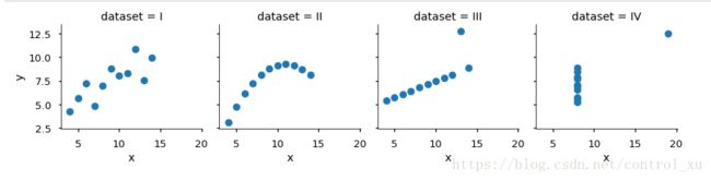
可以看到均值,方差,相关性都相等。线性回归的结果也相同。从Part2的练习就可以看到图表的重要性了。
Part 2
Using Seaborn, visualize all four datasets.
hint: use sns.FacetGrid combined with plt.scatter
如hint所说的,调用这两个函数即可。但是注意第一个形成Grid的时候需要使用dataset为(标签?)
g = sns.FacetGrid(anascombe, col = 'dataset')
g_map = g.map(plt.scatter, 'x', 'y')
结果如下