Python学习——matplotlib作业

Matplotlib Exercises

Exercise 11.1: Plotting a function

Plot the function

f(x)=sin2(x−2)e−x2 f ( x ) = s i n 2 ( x − 2 ) e − x 2

over the interval [0, 2]. Add proper axis labels, a title, etc.

def func(nums):
    return (np.sin(nums - 2) ** 2) * (np.e ** (-nums ** 2))

X = np.linspace(0, 2, 50)
Y = func(X)
ax.plot(X, Y)
ax.set_xlabel('x')
ax.set_ylabel('y')
ax.set_xlim(0, 2)
ax.set_ylim(0, 1)
plt.show()

Exercise 11.2: Data

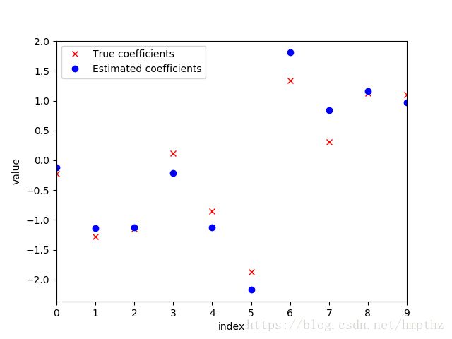
Create a data matrix X with 20 observations of 10 variables. Generate a vector b with parameters Then generate the response vector y = Xb+z where z is a vector with standard normally distributed variables.
Now (by only using y and X), find an estimator for b, by solving

b^=argminb||Xb−y||2 b ^ = a r g min b | | X b − y | | 2

Plot the true parameters b and estimated parameters b^ b ^ . See Figure 1 for an example plot.

分析：用公式

argminx||Ax−b||2=(ATA)−1ATb a r g min x | | A x − b | | 2 = ( A T A ) − 1 A T b

则 b^=(XTX)−1XTy b ^ = ( X T X ) − 1 X T y

def func(X, y):
    tmp1 = np.linalg.inv(np.dot(X.T, X))
    tmp2 = np.dot(X.T, y)
    return np.dot(tmp1, tmp2)

IDX = np.arange(10)
X = np.random.randn(20, 10)
b_True = np.random.randint(-1999, 1999, 10) / 1000.0
z = np.random.randn(20)
y = np.dot(X, b_True) + z
b_Est = func(X, y)

ax.plot(IDX, b_True, 'rx', label='True coefficients')
ax.plot(IDX, b_Est, 'bo', label='Estimated coefficients')
ax.set_xlabel('index')
ax.set_ylabel('value')
ax.set_xlim(0, 9)
ax.legend(loc=0)
plt.show()

Exercise 11.3: Histogram and density estimation

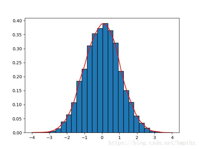
Generate a vector z of 10000 observations from your favorite exotic distribution. Then make a plot that shows a histogram of z (with 25 bins), along with an estimate for the density, using a Gaussian kernel density estimator (see scipy.stats). See Figure 2 for an example plot.

from scipy import stats

z = np.random.randn(10000)
x = np.linspace(-4, 4, 1000)
kernel_z = stats.gaussian_kde(z)
eval_z = kernel_z.pdf(x)
ax.hist(z, bins=25, density=True, edgecolor='k')
ax.plot(x, eval_z, 'r', lw=1.5)
plt.show()