一。神经网络程序快速体验
1.神经网络使用方式
网络结构文件(*.prototxt) 和训练数据集 -> 训练网络(caffe)->网络权重文件(*.caffemodel) 和网络结构文件 -> cuda程序(部署框架caffe和tensorRT)
2.部署框架tensorRT
TensorRT采取“精度换速度的”策略,在精度无明显下降的前提下,其对 inference 的加速明显,往往有1倍以上的性能提升。它能根据 prototxt 文件和 caffemodel 权值,
转化为支持半精度的新的模型。其工作流程如下:
构建阶段:构建一个网络,执行优化
执行阶段:引擎运行推理任务
3.CUDA程序体验
a。安装一下cuda
b。参考链接
https://github.com/dusty-nv/jetson-inference#system-setup 进行cuda程序的下载。
https://github.com/dusty-nv/jetson-inference#locating-object-coordinates-using-detectnet
Cloning the Repo
To obtain the repository, navigate to a folder of your choosing on the Jetson. First, make sure git and cmake are installed locally:
$ sudo apt-get install git cmake
Then clone the jetson-inference repo:
$ git clone http://github.com/dusty-nv/jetson-inference
Configuring with CMake
When cmake is run, a special pre-installation script (CMakePreBuild.sh) is run and will automatically install any dependencies.
$ cd jetson-inference
$ mkdir build
$ cd build
$ cmake ../
note: the cmake command will launch the CMakePrebuild.sh script which asks for sudo while making sure prerequisite packages have been installed on the Jetson. The script also downloads the network model snapshots from web services.
Compiling the Project
Make sure you are still in the jetson-inference/build directory, created above in step #2.
$ cd jetson-inference/build			# omit if pwd is already /build from above
$ make
Depending on architecture, the package will be built to either armhf or aarch64, with the following directory structure:
|-build
   \aarch64		    (64-bit)
      \bin			where the sample binaries are built to
      \include		where the headers reside
      \lib			where the libraries are build to
   \armhf           (32-bit)
      \bin			where the sample binaries are built to
      \include		where the headers reside
      \lib			where the libraries are build to
binaries residing in aarch64/bin, headers in aarch64/include, and libraries in aarch64/lib.
Digging Into the Code
For reference, see the available vision primitives, including imageNet for image recognition and detectNet for object localization.
/**
 * Image recognition with GoogleNet/Alexnet or custom models, using TensorRT.
 */
class imageNet : public tensorNet { public: /**  * Network choice enumeration.  */ enum NetworkType { ALEXNET, GOOGLENET }; /**  * Load a new network instance  */ static imageNet* Create( NetworkType networkType=GOOGLENET ); /**  * Load a new network instance  * @param prototxt_path File path to the deployable network prototxt  * @param model_path File path to the caffemodel  * @param mean_binary File path to the mean value binary proto  * @param class_info File path to list of class name labels  * @param input Name of the input layer blob.  */ static imageNet* Create( const char* prototxt_path, const char* model_path, const char* mean_binary, const char* class_labels, const char* input="data", const char* output="prob" ); /**  * Determine the maximum likelihood image class.  * @param rgba float4 input image in CUDA device memory.  * @param width width of the input image in pixels.  * @param height height of the input image in pixels.  * @param confidence optional pointer to float filled with confidence value.  * @returns Index of the maximum class, or -1 on error.  */ int Classify( float* rgba, uint32_t width, uint32_t height, float* confidence=NULL ); };
Both inherit from the shared tensorNet object which contains common TensorRT code.
Classifying Images with ImageNet
There are multiple types of deep learning networks available, including recognition, detection/localization, and soon segmentation. The first deep learning capability we're highlighting in this tutorial is image recognition using an 'imageNet' that's been trained to identify similar objects.
The imageNet object accepts an input image and outputs the probability for each class. Having been trained on ImageNet database of 1000 objects, the standard AlexNet and GoogleNet networks are downloaded during step 2 from above. As examples of using imageNet we provide a command-line interface called imagenet-console and a live camera program called imagenet-camera.
Using the Console Program on Jetson
First, try using the imagenet-console program to test imageNet recognition on some example images. It loads an image, uses TensorRT and the imageNet class to perform the inference, then overlays the classification and saves the output image.
After building, make sure your terminal is located in the aarch64/bin directory:
$ cd jetson-inference/build/aarch64/bin
Then, classify an example image with the imagenet-console program. imagenet-console accepts 2 command-line arguments: the path to the input image and path to the output image (with the class overlay printed).
$ ./imagenet-console orange_0.jpg output_0.jpg
$ ./imagenet-console granny_smith_1.jpg output_1.jpg
Next, we will use imageNet to classify a live video feed from the Jetson onboard camera.
Running the Live Camera Recognition Demo
Similar to the last example, the realtime image recognition demo is located in /aarch64/bin and is called imagenet-camera. It runs on live camera stream and depending on user arguments, loads googlenet or alexnet with TensorRT.
$ ./imagenet-camera googlenet           # to run using googlenet
$ ./imagenet-camera alexnet             # to run using alexnet
The frames per second (FPS), classified object name from the video, and confidence of the classified object are printed to the openGL window title bar. By default the application can recognize up to 1000 different types of objects, since Googlenet and Alexnet are trained on the ILSVRC12 ImageNet database which contains 1000 classes of objects. The mapping of names for the 1000 types of objects, you can find included in the repo under data/networks/ilsvrc12_synset_words.txt
note: by default, the Jetson's onboard CSI camera will be used as the video source. If you wish to use a USB webcam instead, change the
DEFAULT_CAMERAdefine at the top ofimagenet-camera.cppto reflect the /dev/video V4L2 device of your USB camera. The model it's tested with is Logitech C920.
Re-training the Network with DIGITS
The existing GoogleNet and AlexNet models that are downloaded by the repo are pre-trained on 1000 classes of objects from the ImageNet ILSVRC12 benchmark.
To recognize a new object class, you can use DIGITS to re-train the network on new data. You can also organize the existing classes differently, including group multiple subclasses into one. For example in this tutorial we'll take 230 of the 1000 classes, group those into 12 classes and retrain the network.
Let's start by downloading the ILSVRC12 images to work with, or you can substitute your own dataset in an Image Folder.
Downloading Image Recognition Dataset
An image recognition dataset consists of a large number of images sorted by their classification type (typically by directory). The ILSVRC12 dataset was used in the training of the default GoogleNet and AlexNet models. It's roughly 100GB in size and includes 1 million images over 1000 different classes. The dataset is downloaded to the DIGITS server using the imagenet-download.pyimage crawler.
To download the dataset, first make sure you have enough disk space on your DIGITS server (120GB recommended), then run the following commands from a directory on that machine where you want the dataset stored:
$ wget --no-check-certificate https://nvidia.box.com/shared/static/gzr5iewf5aouhc5exhp3higw6lzhcysj.gz -O ilsvrc12_urls.tar.gz
$ tar -xzvf ilsvrc12_urls.tar.gz
$ wget https://rawgit.com/dusty-nv/jetson-inference/master/tools/imagenet-download.py
$ python imagenet-download.py ilsvrc12_urls.txt . --jobs 100 --retry 3 --sleep 0
In the commands above the list of image URLs along with the scripts are downloaded before launching the crawler.
note: be considerate running the image crawler from a corporate network, IT may flag the activity. It will probably take overnight on a decent connection to download the 1000 ILSVRC12 classes (100GB).
The crawler will download images to subdirectories that correspond to it's classification. Each image class is stored in it's own directory, with 1000 directories in total (one for each class in ILSVRC12). The folders are organized with a naming scheme similar to:
n01440764/
n01443537/
n01484850/
n01491361/
n01494475/
...
These 8-digit ID's prefixed wth N are referred to as the synset ID of the class. The name string of the class can be looked up in ilsvrc12_synset_words.txt. For example, synset n01484850 great white shark.
Customizing the Object Classes
The dataset that we downloaded in the previous step was used to train the default AlexNet and GoogleNet models with 1000 object classes from several core groups, including different species of birds, plants, fruit, and fish, dog and cat breeds, types of vehicles, ect. For practicle purposes lets consider a companion to the GoogleNet model which recognizes a dozen core groups made up of the original 1000 classes (for example, instead of detecting 122 individual breeds of dogs, combining them all into one common dog class). These 12 core groups may be more practical to use than 1000 individual synsets and combining across classes results in more training data and stronger classification for the group.
DIGITS expects the data in a hierarchy of folders, so we can create directories for the groups and then symbolically link to the synsets from ILSVRC12 downloaded above. DIGITS will automatically combine images from all folders under the top-level groups. The directory structure resembles the following, with the value in parenthesis indicates the number of classes used to make up the group and the value next to the arrows indicating the synset ID linked to.
‣ ball/  (7)
	• baseball     (→n02799071)
	• basketball   (→n02802426)
	• soccer ball  (→n04254680)
	• tennis ball  (→n04409515)
	• ...
‣ bear/  (4)
	• brown bear   (→n02132136)
	• black bear   (→n02133161)
	• polar bear   (→n02134084)
	• sloth bear   (→n02134418)
• bike/  (3)
• bird/  (17)
• bottle/ (7)
• cat/  (13)
• dog/  (122)
• fish/   (5)
• fruit/  (12)
• turtle/  (5)
• vehicle/ (14)
• sign/  (2)
Since there are actually a lot of synsets linked to from ILSVRC12, we provide the imagenet-subset.sh script to generate the directory structure and links given the path to the dataset. Run the folowing commands from the DIGITS server:
$ wget https://rawgit.com/dusty-nv/jetson-inference/master/tools/imagenet-subset.sh
$ chmod +x imagenet-subset.sh
$ mkdir 12_classes
$ ./imagenet-subset.sh /opt/datasets/imagenet/ilsvrc12 12_classes
In this example the links are created in the 12_classes folder, with the first argument to the script being the path to ILSVRC12 downloaded in the previous step.
Importing Classification Dataset into DIGITS
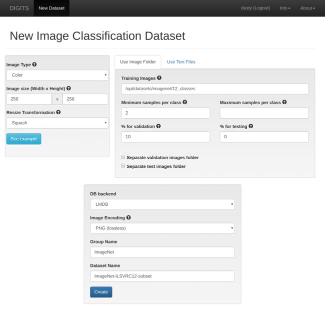
Navigate your browser to your DIGITS server instance and choose to create a new Classification Dataset from the drop-down under the Datasets tab:
Set the Training Images path to the 12_classes folder from the previous step and make the following
- % for validation:
10 - Group Name:
ImageNet - Dataset Name:
ImageNet-ILSVRC12-subset
Use the Create button at the bottom of the page to launch the dataset import job. The size of the data subset is around 20GB, so depending on server I/O performance it takes 10-15 minutes. Next we'll create the new model and begin training it.
Creating Image Classification Model with DIGITS
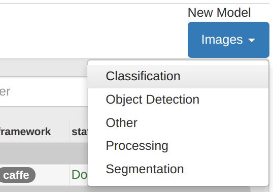
When the previous data import job is complete, return to the DIGITS home screen. Select the Models tab and choose to create a new Classification Model from the drop-down:
Make the following settings in the form:
- Select Dataset:
ImageNet-ILSVRC12-subset - Subtract Mean:
Pixel - Standard Networks:
GoogleNet - Group Name:
ImageNet - Model Name:
GoogleNet-ILSVRC12-subset
After selecting a GPU to train on, click the Create button at the bottom to begin training.
Testing Classification Model in DIGITS
After the training job completes 30 epochs, the trained model should appear like so:
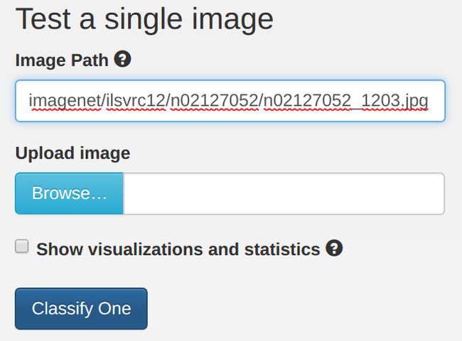
At this point, we can try testing our new model's inference on some example images in DIGITS. On the same page as the plot above, scroll down under the Trained Models section. Under Test a Single Image, select an image to try (for example, /ilsvrc12/n02127052/n02127052_1203.jpg):
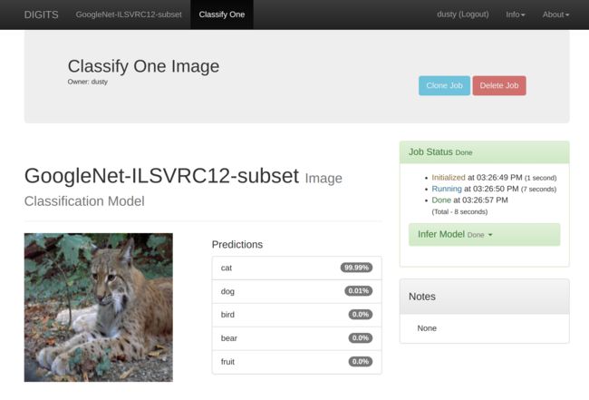
Press the Classify One button and you should see a page similar to:
The image is classified as the new GoogleNet-12 model as cat, while in the original GoogleNet-1000 it was under Lynx. This indicates the new model is working ok, because the Lynx category was included in GoogleNet-12's training of cat.
Downloading Model Snapshot to Jetson
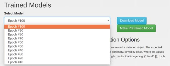
Now that we confirmed the trained model is working in DIGITS, let's download and extract the model snapshot to Jetson. From the browser on your Jetson TX1/TX2, navigate to your DIGITS server and the GoogleNet-ILSVRC12-subset model. Under the Trained Models section, select the desired snapshot from the drop-down (usually the one with the highest epoch) and click the Download Model button.
Alternatively, if your Jetson and DIGITS server aren't accessible from the same network, you can use the step above to download the snapshot to an intermediary machine and then use SCP or USB stick to copy it to Jetson.
Then extract the archive with a command similar to:
tar -xzvf 20170524-140310-8c0b_epoch_30.0.tar.gz
Next we will load our custom snapshot into TensorRT, running on the Jetson.
Loading Custom Models on Jetson
The imagenet-console and imagenet-camera programs that we used before also accept extended command line parameters for loading a custom model snapshot. Set the $NET variable below to the path to your extracted snapshot:
$ NET=networks/GoogleNet-ILSVRC12-subset

$ ./imagenet-console bird_0.jpg output_0.jpg \
--prototxt=$NET/deploy.prototxt \
--model=$NET/snapshot_iter_184080.caffemodel \
--labels=$NET/labels.txt \
--input_blob=data \
--output_blob=softmax
As before, the classification and confidence will be overlayed to the output image. When compared to the output of the original network, the re-trained GoogleNet-12 makes similar classifications to the original GoogleNet-1000:
The extended command line parameters above also load custom classification models with imagenet-camera.
Locating Object Coordinates using DetectNet
The previous image recognition examples output class probabilities representing the entire input image. The second deep learning capability we're highlighting in this tutorial is detecting objects, and finding where in the video those objects are located (i.e. extracting their bounding boxes). This is performed using a 'detectNet' - or object detection / localization network.
The detectNet object accepts as input the 2D image, and outputs a list of coordinates of the detected bounding boxes. To train the object detection model, first a pretrained ImageNet recognition model (like Googlenet) is used with bounding coordinate labels included in the training dataset in addition to the source imagery.
The following pretrained DetectNet models are included with the tutorial:
- ped-100 (single-class pedestrian detector)
- multiped-500 (multi-class pedestrian + baggage detector)
- facenet-120 (single-class facial recognition detector)
- coco-airplane (MS COCO airplane class)
- coco-bottle (MS COCO bottle class)
- coco-chair (MS COCO chair class)
- coco-dog (MS COCO dog class)
As with the previous examples, provided are a console program and a camera streaming program for using detectNet.
Detection Data Formatting in DIGITS
Example object detection datasets with include KITTI, MS-COCO, and others. To use the KITTI dataset follow this DIGITS object detection tutorial with KITTI.
Regardless of dataset, DIGITS uses KITTI metadata format for ingesting the detection bounding labels. These consist of text files with frame numbers corresponding to image filenames, including contents such as:
dog 0 0 0 528.63 315.22 569.09 354.18 0 0 0 0 0 0 0
sheep 0 0 0 235.28 300.59 270.52 346.55 0 0 0 0 0 0 0
Read more about the folder structure and KITTI label format that DIGITS uses.
Downloading the Detection Dataset
Let's explore using the MS-COCO dataset to train and deploy networks that detect the locations of everyday objects in camera feeds. See the coco2kitti.py script for converting MS-COCO object classes to KITTI format. Once in DIGITS folder structure, they can be imported as datasets into DIGITS. Some example classes from MS-COCO already preprocessed in DIGITS/KITTI format are provided for convienience.
From a terminal on your DIGITS server download and extract sample MS-COCO classes already in DIGITS/KITTI format here:
$ wget --no-check-certificate https://nvidia.box.com/shared/static/tdrvaw3fd2cwst2zu2jsi0u43vzk8ecu.gz -O coco.tar.gz

HTTP request sent, awaiting response... 200 OK
Length: 5140413391 (4.5G) [application/octet-stream]
Saving to: ‘coco.tar.gz’

coco 100%[======================================>]   4.5G  3.33MB/s    in 28m 22s

2017-04-17 10:41:19 (2.5 MB/s) - ‘coco.tar.gz’ saved [5140413391/5140413391]

$ tar -xzvf coco.tar.gz
Included is the training data in DIGITS format for the airplane, bottle, chair, and dog classes. coco2kitti.py can be used to convert other classes.
Importing the Detection Dataset into DIGITS
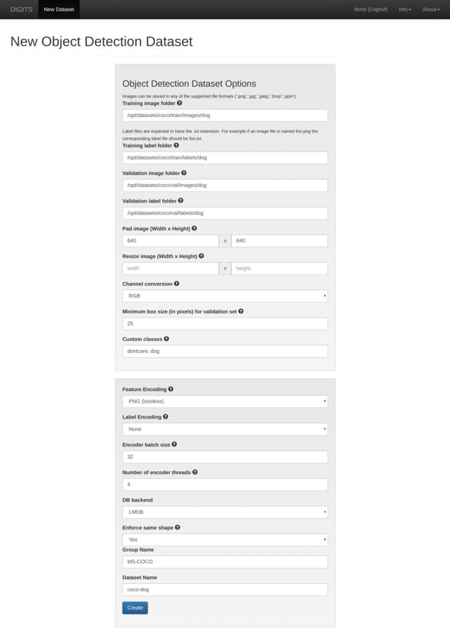
Navigate your browser to your DIGITS server instance and choose to create a new Detection Dataset from the drop-down in the Datasets tab:
In the form fields, specify the following options and paths to the image and label folders under the location where you extracted the aerial dataset:
- Training image folder:
coco/train/images/dog - Training label folder:
coco/train/labels/dog - Validation image folder:
coco/val/images/dog - Validation label folder:
coco/val/labels/dog - Pad image (Width x Height):
640 x 640 - Custom classes:
dontcare, dog - Group Name:
MS-COCO - Dataset Name:
coco-dog
Name the dataset whatever you choose and click the Create button at the bottom of the page to launch the importing job. Next we'll create the new detection model and begin training it.
Creating DetectNet Model with DIGITS
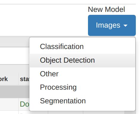
When the previous data import job is complete, return to the DIGITS home screen. Select the Models tab and choose to create a new Detection Model from the drop-down:
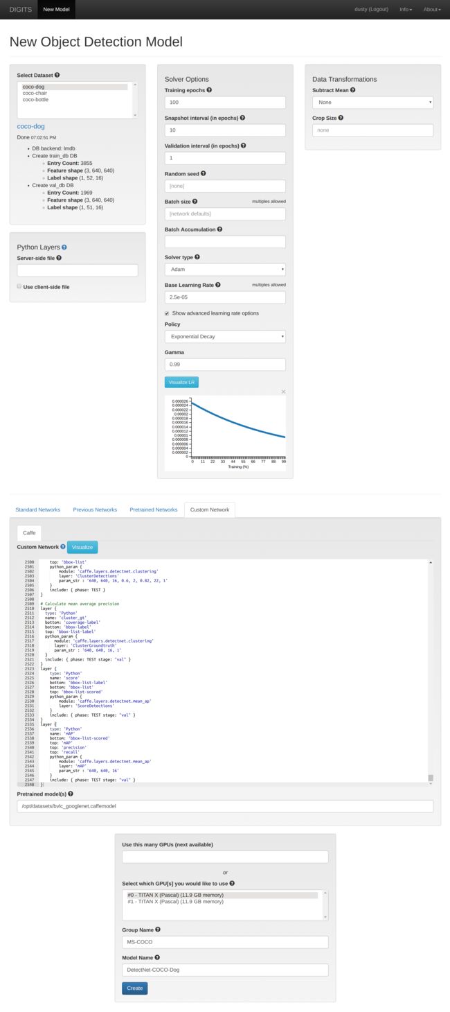
Make the following settings in the form:
- Select Dataset:
coco-dog - Training epochs:
100 - Subtract Mean:
none - Solver Type:
Adam - Base learning rate:
2.5e-05 - Select
Show advanced learning options- Policy:
Exponential Decay - Gamma:
0.99
- Policy:
Selecting DetectNet Batch Size
DetectNet's network default batch size of 10 consumes up to 12GB GPU memory during training. However by using the Batch Accumulation field, you can also train DetectNet on a GPU with less than 12GB memory. See the table below depending on the amount of GPU memory available in your DIGITS server:
| GPU Memory | Batch Size | Batch Accumulation |
|---|---|---|
| 4GB | 2 | 5 |
| 8GB | 5 | 2 |
| 12GB or larger | [network defaults] (10) |
Leave blank (1) |
If you're training on a card with 12GB of memory or more, leave the Batch Size as the default and leave the Batch Accumulation blank. For GPUs with less memory, use the settings from above.
Specifying the DetectNet Prototxt
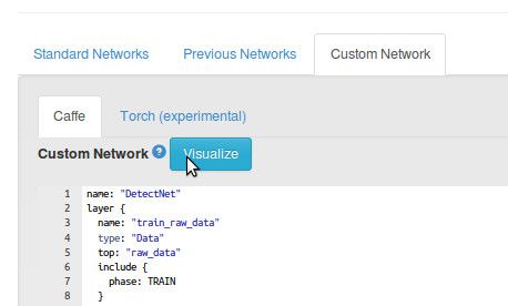
In the network area select the Custom Network tab and then copy/paste the contents of detectnet.prototxt
The DetectNet prototxt is located at data/networks/detectnet.prototxt in the repo.
Training the Model with Pretrained Googlenet
Since DetectNet is derived from Googlenet, it is strongly recommended to use pre-trained weights from Googlenet as this will help speed up and stabilize training significantly. Download the Googlenet model from here or by running the following command from your DIGITS server:
wget http://dl.caffe.berkeleyvision.org/bvlc_googlenet.caffemodel
Then specify the path to your Googlenet under the Pretrained Model field.
Select a GPU to train on and set a name and group for the model:
- Group Name
MS-COCO - Model Name
DetectNet-COCO-Dog
Finally, click the Create button at the bottom to begin training.
Testing DetectNet Model Inference in DIGITS
Leave the training job to run for a while, say 50 epochs, until the mAP (Mean Average Precision) plot begins to increase. Note that due to the way mAP is calculated by the DetectNet loss function, the scale of mAP isn't necessarily 0-100, and even an mAP between 5 and 10 may indicate the model is functional. With the size of the example COCO datasets we are using, it should take a couple hours training on a recent GPU before all 100 epochs are complete.
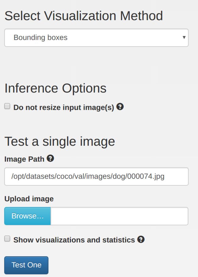
At this point, we can try testing our new model's inference on some example images in DIGITS. On the same page as the plot above, scroll down under the Trained Models section. Set the Visualization Model to Bounding Boxes and under Test a Single Image, select an image to try (for example, /coco/val/images/dog/000074.png):
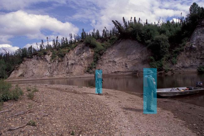
Press the Test One button and you should see a page similar to:
Downloading the Model Snapshot to Jetson
Next, download and extract the trained model snapshot to Jetson. From the browser on your Jetson TX1/TX2, navigate to your DIGITS server and the DetectNet-COCO-Dog model. Under the Trained Models section, select the desired snapshot from the drop-down (usually the one with the highest epoch) and click the Download Model button.
Alternatively, if your Jetson and DIGITS server aren't accessible from the same network, you can use the step above to download the snapshot to an intermediary machine and then use SCP or USB stick to copy it to Jetson.
Then extract the archive with a command similar to:
tar -xzvf 20170504-190602-879f_epoch_100.0.tar.gz
DetectNet Patches for TensorRT
In the original DetectNet prototxt exists a Python clustering layer which isn't available in TensorRT and should be deleted from the deploy.prototxt included in the snapshot. In this repo the detectNet class handles the clustering as opposed to Python.
At the end of deploy.prototxt, delete the layer named cluster:
layer {
  name: "cluster"
  type: "Python"
  bottom: "coverage"
  bottom: "bboxes"
  top: "bbox-list"
  python_param {
    module: "caffe.layers.detectnet.clustering"
    layer: "ClusterDetections"
    param_str: "640, 640, 16, 0.6, 2, 0.02, 22, 1"
  }
}
Without this Python layer, the snapshot can now be imported into TensorRT.
Processing Images from the Command Line on Jetson
To process test images with detectNet and TensorRT, use the detectnet-console program. detectnet-console accepts command-line arguments representing the path to the input image and path to the output image (with the bounding box overlays rendered). Some test images are also included with the repo.
To specify your model that you downloaded from DIGITS, use the syntax to detectnet-console below. First, for convienience, set the path to your extracted snapshot into a $NET variable:
$ NET=20170504-190602-879f_epoch_100

$ ./detectnet-console dog_0.jpg output_0.jpg \
--prototxt=$NET/deploy.prototxt \
--model=$NET/snapshot_iter_38600.caffemodel \
--input_blob=data \
--output_cvg=coverage \
--output_bbox=bboxes
note: the
input_blob,output_cvg, andoutput_bboxarguments may be omitted if your DetectNet layer names match the defaults above (i.e. if you are using the prototxt from following this tutorial). These optional command line parameters are provided if you are using a customized DetectNet with different layer names.
Launching With a Pretrained Model
Alternatively, to load one of the pretrained snapshots that comes with the repo, you can specify the pretrained model name as the 3rd argument to detectnet-console:
$ ./detectnet-console dog_1.jpg output_1.jpg coco-dog
The above command will process dog_1.jpg, saving it to output_1.jpg, using the pretrained DetectNet-COCO-Dog model. This is a shortcut of sorts so you don't need to wait for the model to complete training if you don't want to.
Pretrained DetectNet Models Available
Below is a table of the pretrained DetectNet snapshots downloaded with the repo (located in the data/networks directory after running cmake step) and the associated argument to detectnet-console used for loading the pretrained model:
| DIGITS model | CLI argument | classes |
|---|---|---|
| DetectNet-COCO-Airplane | coco-airplane |
airplanes |
| DetectNet-COCO-Bottle | coco-bottle |
bottles |
| DetectNet-COCO-Chair | coco-chair |
chairs |
| DetectNet-COCO-Dog | coco-dog |
dogs |
| ped-100 | pednet |
pedestrians |
| multiped-500 | multiped |
pedestrians, luggage |
| facenet-120 | facenet |
faces |
These all also have the python layer patch above already applied.
Running Other MS-COCO Models on Jetson
Let's try running some of the other COCO models. The training data for these are all included in the dataset downloaded above. Although the DIGITS training example above was for the coco-dog model, the same procedure can be followed to train DetectNet on the other classes included in the sample COCO dataset.
$ ./detectnet-console bottle_0.jpg output_2.jpg coco-bottle
$ ./detectnet-console airplane_0.jpg output_3.jpg coco-airplane
Running Pedestrian Models on Jetson
Included in the repo are also DetectNet models pretrained to detect humans. The pednet and multiped models recognized pedestrians while facenet recognizes faces (from FDDB). Here's an example of detecting multiple humans simultaneously in a crowded space:
$ ./detectnet-console peds-004.jpg output-4.jpg multiped
Multi-class Object Detection Models
When using the multiped model (PEDNET_MULTI), for images containing luggage or baggage in addition to pedestrians, the 2nd object class is rendered with a green overlay.
$ ./detectnet-console peds-003.jpg output-3.jpg multiped
Running the Live Camera Detection Demo on Jetson
Similar to the previous example, detectnet-camera runs the object detection networks on live video feed from the Jetson onboard camera. Launch it from command line along with the type of desired network:
$ ./detectnet-camera coco-bottle    # detect bottles/soda cans in the camera
$ ./detectnet-camera coco-dog       # detect dogs in the camera
$ ./detectnet-camera multiped       # run using multi-class pedestrian/luggage detector $ ./detectnet-camera pednet # run using original single-class pedestrian detector $ ./detectnet-camera facenet # run using facial recognition network $ ./detectnet-camera # by default, program will run using multiped
note: to achieve maximum performance while running detectnet, increase the Jetson clock limits by running the script:
sudo ~/jetson_clocks.sh
note: by default, the Jetson's onboard CSI camera will be used as the video source. If you wish to use a USB webcam instead, change the
DEFAULT_CAMERAdefine at the top ofdetectnet-camera.cppto reflect the /dev/video V4L2 device of your USB camera and recompile. The webcam model it's tested with is Logitech C920.
Image Segmentation with SegNet
The third deep learning capability we're highlighting in this tutorial is image segmentation. Segmentation is based on image recognition, except the classifications occur at the pixel level as opposed to classifying entire images as with image recognition. This is accomplished by convolutionalizing a pre-trained imageNet recognition model (like Alexnet), which turns it into a fully-convolutional segmentation model capable of per-pixel labelling. Useful for environmental sensing and collision avoidance, segmentation yields dense per-pixel classification of many different potential objects per scene, including scene foregrounds and backgrounds.
The segNet object accepts as input the 2D image, and outputs a second image with the per-pixel classification mask overlay. Each pixel of the mask corresponds to the class of object that was classified.
note: see the DIGITS semantic segmentation example for more background info on segmentation.
Downloading Aerial Drone Dataset
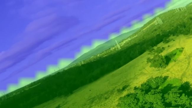
As an example of image segmentation, we'll work with an aerial drone dataset that separates ground terrain from the sky. The dataset is in First Person View (FPV) to emulate the vantage point of a drone in flight and train a network that functions as an autopilot guided by the terrain that it senses.
To download and extract the dataset, run the following commands from the host PC running the DIGITS server:
$ wget --no-check-certificate https://nvidia.box.com/shared/static/ft9cc5yjvrbhkh07wcivu5ji9zola6i1.gz -O NVIDIA-Aerial-Drone-Dataset.tar.gz

HTTP request sent, awaiting response... 200 OK
Length: 7140413391 (6.6G) [application/octet-stream]
Saving to: ‘NVIDIA-Aerial-Drone-Dataset.tar.gz’

NVIDIA-Aerial-Drone-Datase 100%[======================================>]   6.65G  3.33MB/s    in 44m 44s

2017-04-17 14:11:54 (2.54 MB/s) - ‘NVIDIA-Aerial-Drone-Dataset.tar.gz’ saved [7140413391/7140413391]

$ tar -xzvf NVIDIA-Aerial-Drone-Dataset.tar.gz
The dataset includes various clips captured from flights of drone platforms, but the one we'll be focusing on in this tutorial is under FPV/SFWA. Next we'll create the training database in DIGITS before training the model.
Importing the Aerial Dataset into DIGITS
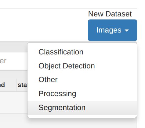
First, navigate your browser to your DIGITS server instance and choose to create a new Segmentation Dataset from the drop-down in the Datasets tab:
In the dataset creation form, specify the following options and paths to the image and label folders under the location where you extracted the aerial dataset:
- Feature image folder:
NVIDIA-Aerial-Drone-Dataset/FPV/SFWA/720p/images - Label image folder:
NVIDIA-Aerial-Drone-Dataset/FPV/SFWA/720p/labels - set
% for validationto 1% - Class labels:
NVIDIA-Aerial-Drone-Dataset/FPV/SFWA/fpv-labels.txt - Color map: From text file
- Feature Encoding:
None - Label Encoding:
None
Name the dataset whatever you choose and click the Create button at the bottom of the page to launch the importing job. Next we'll create the new segmentation model and begin training.
Generating Pretrained FCN-Alexnet
Fully Convolutional Network (FCN) Alexnet is the network topology that we'll use for segmentation models with DIGITS and TensorRT. See this Parallel ForAll article about the convolutionalizing process. A new feature to DIGITS5 was supporting segmentation datasets and training models. A script is included with the DIGITS semantic segmentation example which converts the Alexnet model into FCN-Alexnet. This base model is then used as a pre-trained starting point for training future FCN-Alexnet segmentation models on custom datasets.
To generate the pre-trained FCN-Alexnet model, open a terminal, navigate to the DIGITS semantic-segmantation example, and run the net_surgery script:
$ cd DIGITS/examples/semantic-segmentation
$ ./net_surgery.py
Downloading files (this might take a few minutes)...
Downloading https://raw.githubusercontent.com/BVLC/caffe/rc3/models/bvlc_alexnet/deploy.prototxt...
Downloading http://dl.caffe.berkeleyvision.org/bvlc_alexnet.caffemodel...
Loading Alexnet model...
...
Saving FCN-Alexnet model to fcn_alexnet.caffemodel
Training FCN-Alexnet with DIGITS
When the previous data import job is complete, return to the DIGITS home screen. Select the Models tab and choose to create a new Segmentation Model from the drop-down:
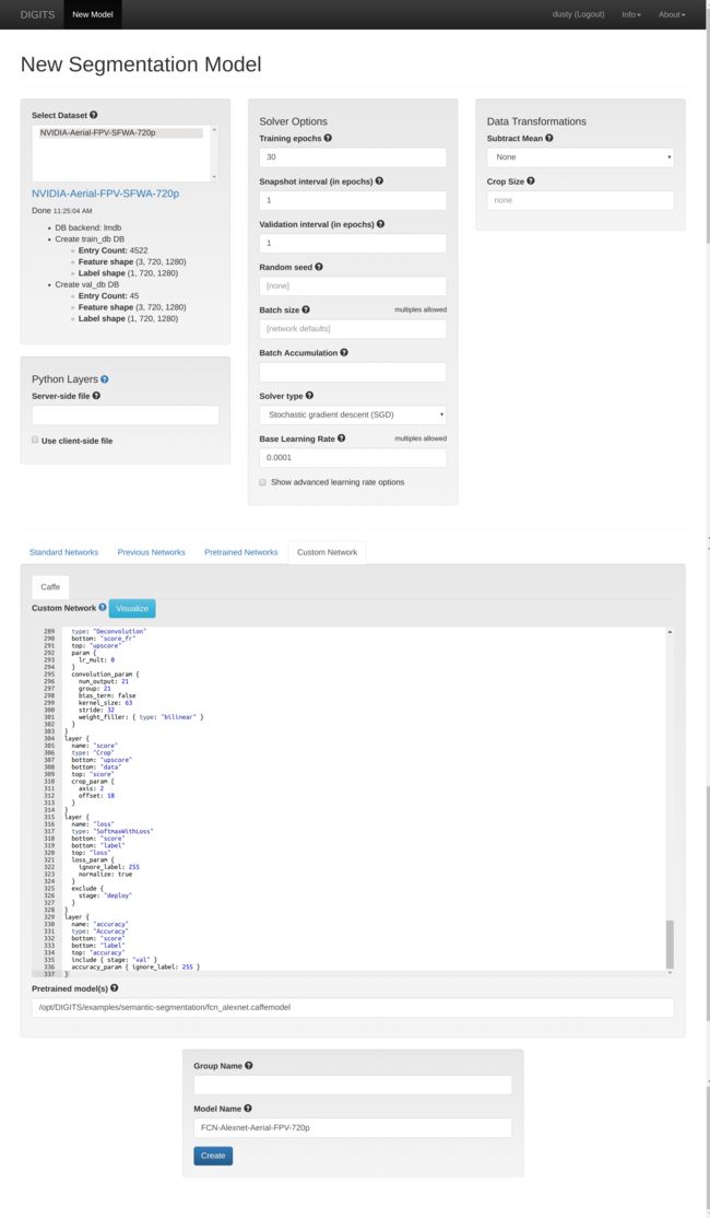
In the model creation form, select the dataset you previously created. Set Subtract Mean to None and the Base Learning Rate to 0.0001. To set the network topology in DIGITS, select the Custom Network tab and make sure the Caffe sub-tab is selected. Copy/paste the FCN-Alexnet prototxt into the text box. Finally, set the Pretrained Model to the output that the net_surgery generated above: DIGITS/examples/semantic-segmentation/fcn_alexnet.caffemodel
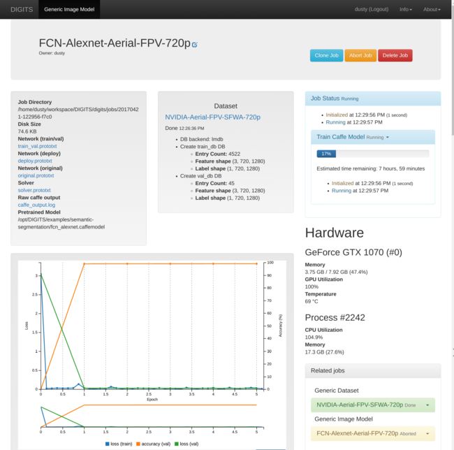
Give your aerial model a name and click the Create button at the bottom of the page to start the training job. After about 5 epochs, the Accuracy plot (in orange) should ramp up and the model becomes usable:
At this point, we can try testing our new model's inference on some example images in DIGITS.
Testing Inference Model in DIGITS
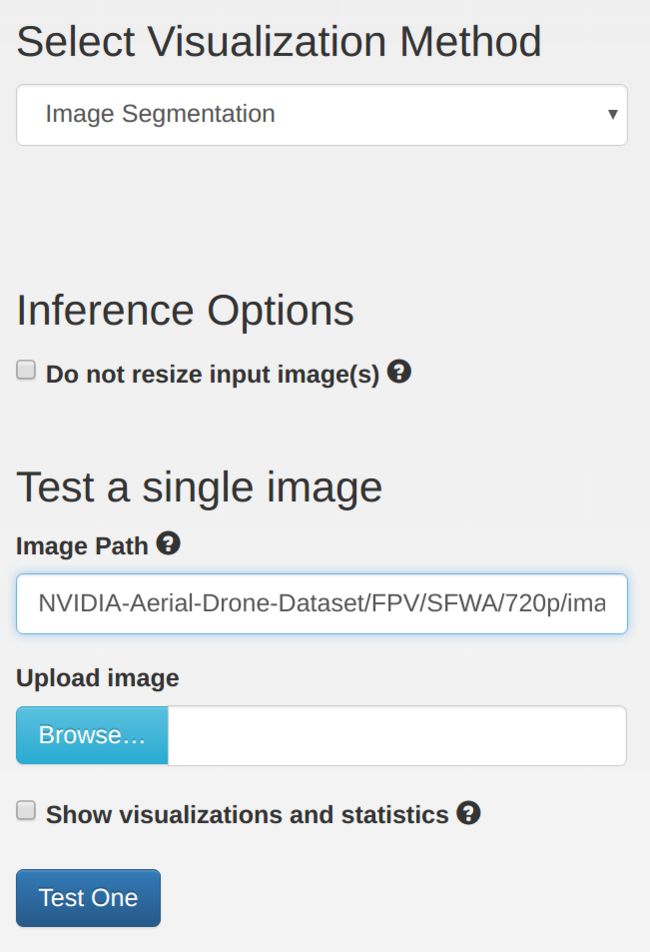
Before transfering the trained model to Jetson, let's test it first in DIGITS. On the same page as previous plot, scroll down under the Trained Models section. Set the Visualization Model to Image Segmentation and under Test a Single Image, select an image to try (for example /NVIDIA-Aerial-Drone-Dataset/FPV/SFWA/720p/images/0428.png):
Press Test One and you should see a display similar to:
Next, download and extract the trained model snapshot to Jetson.
FCN-Alexnet Patches for TensorRT
There exist a couple non-essential layers included in the original FCN-Alexnet which aren't supported in TensorRT and should be deleted from the deploy.prototxt included in the snapshot.
At the end of deploy.prototxt, delete the deconv and crop layers:
layer {
  name: "upscore"
  type: "Deconvolution"
  bottom: "score_fr"
  top: "upscore"
  param {
    lr_mult: 0.0
  }
  convolution_param {
    num_output: 21
    bias_term: false
    kernel_size: 63
    group: 21
    stride: 32
    weight_filler {
      type: "bilinear"
    }
  }
}
layer {
  name: "score"
  type: "Crop"
  bottom: "upscore"
  bottom: "data"
  top: "score"
  crop_param {
    axis: 2
    offset: 18
  }
}
And on line 24 of deploy.prototxt, change pad: 100 to pad: 0. Finally copy the fpv-labels.txt and fpv-deploy-colors.txt from the aerial dataset to your model snapshot folder on Jetson. Your FCN-Alexnet model snapshot is now compatible with TensorRT. Now we can run it on Jetson and perform inference on images.
Running Segmentation Models on Jetson
To test a custom segmentation network model snapshot on the Jetson, use the command line interface to test the segnet-console program.
First, for convienience, set the path to your extracted snapshot into a $NET variable:
$ NET=20170421-122956-f7c0_epoch_5.0

$ ./segnet-console drone_0428.png output_0428.png \
--prototxt=$NET/deploy.prototxt \
--model=$NET/snapshot_iter_22610.caffemodel \
--labels=$NET/fpv-labels.txt \
--colors=$NET/fpv-deploy-colors.txt \
--input_blob=data \
--output_blob=score_fr
This runs the specified segmentation model on a test image downloaded with the repo.
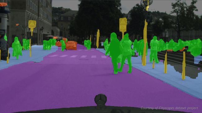
In addition to the pre-trained aerial model from this tutorial, the repo also includes pre-trained models on other segmentation datasets, including Cityscapes, SYNTHIA, and Pascal-VOC.
Extra Resources
In this area, links and resources for deep learning developers are listed:
- Appendix
- NVIDIA Deep Learning Institute — Introductory QwikLabs
- Building nvcaffe
- Other Examples
- ros_deep_learning - TensorRT inference ROS nodes


