英国电商用户行为分析

一.数据的获取

数据集：https://archive.ics.uci.edu/ml/datasets/online+retail#
数据集简介：英国零售在2010.12.1至2011.12.9发生的交易订单
内容：
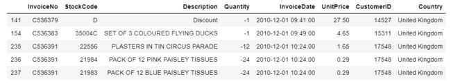
InvoiceNo：发票编号。为每笔订单唯一分配的6位整数。若以字母’C’开头，则表示该订单被取消。
StockCode：产品代码。为每个产品唯一分配的编码。
Description：产品描述。
Quantity：数量。每笔订单中各产品分别的数量。
InvoiceDate：发票日期和时间。每笔订单发生的日期和时间。
UnitPrice：单价。单位产品价格，单位为英镑。
CustomerID：客户编号。为每个客户唯一分配的5位整数。
Country：国家。客户所在国家/地区的名称。

二.读取数据

加载需要用到的库

import numpy as np
import pandas as pd
import matplotlib.pyplot as plt
import seaborn as sns
df_sale =pd.read_excel(r'E:/学习资料/数据分析练习/Online Retail/Online Retail.xlsx')
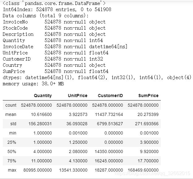
df_sale.info()
df_sale.describe()

共541909条数据，数量和单价均存在负值需要后续处理

三.清洗数据

3.1 删除重复值，观察空值

before = df_sale.shape[0]
df_sale.drop_duplicates(inplace=True)
after = df_sale.shape[0]
print("delete %d duplicated raws"%(before-after))
df_sale.isnull().sum().sort_values(ascending=False)

删除5268行数据，CustomerID 和Description 存在空值
Description 不影响后面的，空值不做处理。同时发现CustomerID为float，做转换int，将空值填充为0，同时将InvoiceNo转换为字符便于‘C’订单的处理

df_sale['CustomerID']=df_sale['CustomerID'].astype('int')
df_sale['InvoiceNo']=df_sale['InvoiceNo'].astype('str')
df_sale.CustomerID.fillna(value=0,inplace=True)

3.2 异常值的处理

df_sale[(df_sale.Quantity<=0)|(df_sale['UnitPrice']<=0)].head()

观察发票号包含C，想到需要将取消的订单与成功的订单分开，应用到正则表达式

query_c= df_sale.InvoiceNo.str.contains("C")
df_cancel =df_sale.loc[query_c,:].copy()
df_sucess =df_sale.loc[-query_c,:].copy()

在成功的订单的中，还要去掉UnitPrice<0的订单，同时考虑到UnitPrice=0可能为活动，也将其去除

query_free =(df_sucess['UnitPrice']==0)
df_sucess= df_sucess.loc[-query_free,:]
query_minus=(df_sucess['UnitPrice']<0)
df_sucess =df_sucess.loc[-query_minus,:]

同时增加总价这列，检查最终的df_sucess数据

df_sucess['SumPrice']=df_sucess.loc[:,'Quantity']* df_sucess.loc[:,'UnitPrice']
df_sucess.info()
df_sucess.describe()

共524878行记录

四.数据分析与可视化（不同维度）

4.1 订单维度：笔单价，连带率

groupInvoiceNo=df_sucess.groupby(r'InvoiceNo')[r'Quantity',r'SumPrice'].agg('sum')
groupInvoiceNo.describe()

笔单价约为533.17英镑，连带率 279件
订单金额与商品件数关系如何？

fig =plt.figure(figsize=(14,4))
sns.distplot(groupInvoiceNo.SumPrice,bins=100,color='c')
plt.title(r'SumPrice distribution of orders')
plt.xticks(np.arange(0,170000,10000))
plt.ylabel(r'Frequency')
plt.grid()
plt.show()

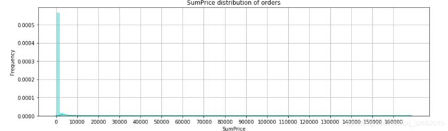
将总金额缩小至2000，进一步观察

fig =plt.figure(figsize=(14,4))
ax= fig.add_subplot(1,1,1)
sns.distplot(groupInvoiceNo.loc[groupInvoiceNo.SumPrice<2000,'SumPrice'],bins=100,color='c',norm_hist=True)
plt.title(r'SumPrice distribution of orders(below 2000)')
plt.ylabel(r'Frequency')
plt.xticks(np.arange(0,2000,100))
plt.grid()
plt.show()

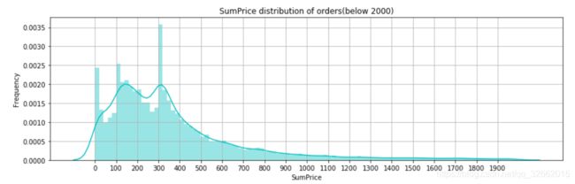
订单金额集中在500英镑内，三个峰值分别为20英镑内、100-120英镑、300-320英镑。其中300-320英镑的订单数量特别多
观察订单商品数量和总价的关系

fig =plt.figure(figsize=(8,8))
plt.subplot(2,1,1)
plt.scatter(x=groupInvoiceNo.Quantity,y=groupInvoiceNo.SumPrice)
plt.xlabel(r'Quantity ')
plt.ylabel(r'SumPrice')
plt.title(r'Quantity & SumPrice')

plt.subplot(2,1,2)
plt.subplots_adjust(hspace=0.5)
plt.scatter(x=groupInvoiceNo.loc[groupInvoiceNo.Quantity<20000,'Quantity'],y=groupInvoiceNo.loc[groupInvoiceNo.Quantity<20000,'SumPrice'])
plt.xlabel(r'Quantity ')
plt.ylabel(r'SumPrice')
plt.title(r'Quantity & SumPrice(Quantity<20000)')
plt.show()

总体来说订单金额和订单中的商品件数为正相关，但是也存在数量极少，总价极高的订单。

4.2客户维度（客单价，客户的消费金额）

df_customer =df_sucess[df_sucess.CustomerID !=0].copy()
group_customer= df_customer.groupby('CustomerID').agg({'Quantity':['sum'],'SumPrice':['sum'],
                                                       'InvoiceNo':lambda x:x.nunique()})
group_customer.columns=['Quantity','SumPrice','InvoiceNo']
group_customer.describe()                                                   

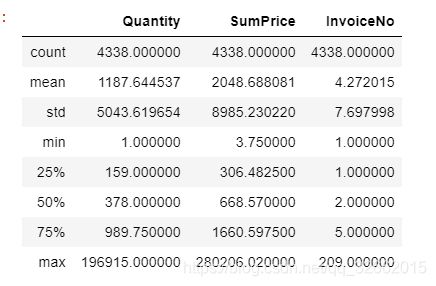
人均购买笔数为4笔，中位数为2笔，25%以上的客户仅下过一次单，并未留存。 每位客户平均购买了1187件商品，甚至超过了Q3分位数，最多的客户购买了196915件；客单价为2049英镑， 平均值同样超过了Q3分位数，说明客户的购买力存在较大差距，存在小部分的高消费用户拉高了人均数值

客户订单总金额的分布

fig =plt.figure(figsize=(7,5))
group_customer.SumPrice.plot.hist(bins=100)
plt.title(r"SumPrice Distribution of Customers")
plt.xlabel(r'SumPrice')
plt.ylabel(r'Frequency')
plt.grid()
plt.show()

fig =plt.figure(figsize=(7,5))
group_customer.loc[group_customer.SumPrice<5000,'SumPrice'].plot.hist(bins=50)
plt.title(r"SumPrice Distribution of Customers(SumPrice<5000)")
plt.xlabel(r'SumPrice')
plt.ylabel(r'Frequency')
plt.xticks(range(0,5000,500))
plt.grid()
plt.show()

与前面订单金额的多峰分布相比，客户消费金额的分布呈现单峰长尾形态，金额更为集中，峰值在100-200英镑间

4.3 商品维度（价格，卖的好，对销售额的贡献）

group_goods =df_sucess.groupby('StockCode').agg({'Quantity':sum,'SumPrice':sum})
group_goods['Average']=group_goods.SumPrice/group_goods.Quantity

所有商品的均价：

fig =plt.figure(figsize=(7,5))
group_goods.Average.hist(bins=100)
plt.xlabel(r'Average Price')
plt.title(r'AvgPrice Distribution')
plt.show()

fig =plt.figure(figsize=(7,5))
group_goods.loc[group_goods.Average<40,'Average'].hist(bins=50)
plt.xlabel(r'Average Price')
plt.title(r'AvgPrice Distribution(Average<40)')
plt.show()

峰值是1-2英磅，单价10磅上的商品已经很少见，该电商的定位主要是价格低区间

fig =plt.figure(figsize=(12,4))
plt.subplot(1,2,1)
plt.scatter(x=group_goods.Average,y=group_goods.Quantity)
plt.title(r'AvgPrice & Quantity')
plt.ylabel(r'Quantity')
plt.xlabel(r'Average Price')
plt.grid()

plt.subplot(1,2,2)
plt.subplots_adjust(wspace=0.5)
plt.scatter(x=group_goods.loc[group_goods.Average<80,'Average'],y=group_goods.loc[group_goods.Average<80,'Quantity'])
plt.title(r'AvgPrice & Quantity(Average<80)')
plt.ylabel(r'Quantity')
plt.xlabel(r'Average Price')
plt.grid()
plt.show()

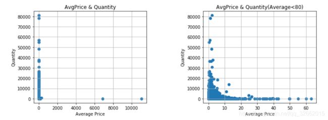
从商品销量看，低于5英镑的低价区商品更受到客户的喜爱`

fig =plt.figure(figsize=(12,5))
plt.subplot(1,2,1)
plt.scatter(x=group_goods.Average,y=group_goods.SumPrice)
plt.title(r'AvgPrice & SumPrice')
plt.ylabel(r'SumPrice')
plt.xlabel(r'Average Price')

plt.subplot(1,2,2)
plt.subplots_adjust(wspace=0.5)
plt.scatter(x=group_goods.loc[group_goods.Average<80,'Average'],y=group_goods.loc[group_goods.Average<80,'SumPrice'])
plt.title(r'AvgPrice & SumPrice(Average<80)')
plt.ylabel(r'SumPrice')
plt.xlabel(r'Average Price')
plt.show()

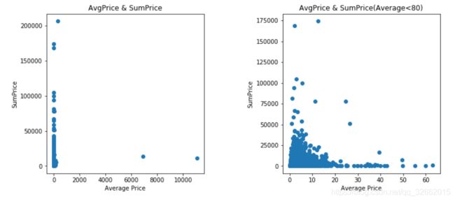
低价区的商品构成了销售额的主要部分，高价的商品虽然单价高昂，并没有带来太多的销售额

4.4 时间维度
对日期进行处理

df_sucess['Month']=df_sucess.InvoiceDate.dt.month
df_sucess['Date']=df_sucess.InvoiceDate.dt.date

按照月份观察销量和总价

group_month=df_sucess.groupby('Month').agg({'InvoiceNo':lambda x:x.nunique(),'SumPrice':sum,'Quantity':sum})
month =group_month.plot(secondary_y ='InvoiceNo', x_compat=True,figsize=(10,5))
month.set_ylabel('Quantity & SumPrice')
month.right_ax.set_ylabel('Order quantities')
month.set_xticks(np.arange(0,12,1))
plt.grid()
plt.show()

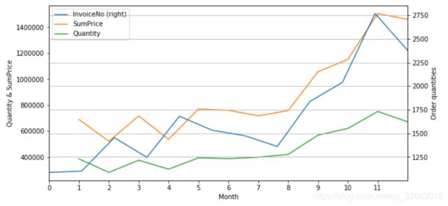
除了2011年2月和4月略低外，2010年12月至2011年8月基本维持相近的销售情况；随后在9月-11月连续增长，达到高峰。考虑该电商平台主营礼品，受节日影响可能较大,欧洲重视的万圣节（11月1日）和圣诞节（12月25日）都在年末，与图中的趋势能够相呼应

group_date =df_sucess.groupby(df_sucess.Date).agg({'InvoiceNo':lambda x: x.nunique(),'SumPrice':sum,'Quantity':sum})

group_date.loc[:,['SumPrice','Quantity']].plot(figsize=(10,5))
plt.title('SumPrice & Quantity & Date')
plt.ylabel(r'SumPrice & Quantity ')

group_date.loc[:,['InvoiceNo']].plot(figsize=(10,5))
plt.ylabel(r'InvoiceNo')
plt.title(r'InvoiceNo & Date')
plt.show()

可见销量Quantity和销售额SumPrice的趋势是极趋同的，这也和前一节中分析出该电商以低价商品为主相吻合，商品单价低且价位集中，则销售额主要随销量变化而涨跌,注意到在最后一天（即2011年12月9日），销量、销售额显著激增

将12月的销售额和销量单独拉出来看

df_sucess.Date =pd.to_datetime(df_sucess.Date,format='%Y-%m-%d')

group_daypart=df_sucess.groupby('Date').agg({'InvoiceNo':lambda x:x.nunique(),'SumPrice':sum,'Quantity':sum})

day_part=group_daypart['2011-12-01':].plot(secondary_y = 'InvoiceNo', figsize = (12,6),legend='best')
day_part.set_ylabel('Quantity & SumPrice')
day_part.right_ax.set_ylabel('Order quantities')
plt.show()

2011年12月的前8天基本延续了11月下旬的销售趋势，但在12月9日订单量大幅下降时，却创造了样本区间内销量和销售额的历史新高。说明存在某笔或某几笔购买量极大的订单，从而使得销售额大幅上升

df_sucess[df_sucess.Date=='2011-12-09'].sort_values(by='SumPrice',ascending =False)[:5]

一个英国的客户，一口气购买了8万余件的纸工艺品，贡献了168469英镑的销售额

4.5 国家维度

group_country =df_sucess.groupby('Country').agg({'InvoiceNo':lambda x:x.nunique(),'SumPrice':sum })

group_country.sort_values(by='SumPrice',ascending =False)

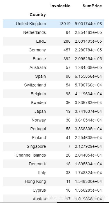
可知绝大部分客户仍来自英国本土，主要境外收入来源也多为英国周边国家,这种现象可能和运输成本及语言等有关，也可能是影响力随距离而衰减，可以尝试增加境外的宣传投放，提高知名度；

4.6 客户行为（生命周期，留存，购买周期）
需要先去除没有CustomerID的用户

df_cust_action =df_sucess[df_sucess.CustomerID !=0].copy()

生命周期，第一次购买和最近购买相减

group_life_cycle=df_cust_action.groupby('CustomerID')['Date'].agg([min,max])
group_life_cycle.columns=['Fst','Last']
group_life_cycle['Lifecycle']=(group_life_cycle['Last']-group_life_cycle['Fst']).dt.days

图表展示：

fig=plt.figure(figsize =(8,5))
plt.hist(x=group_life_cycle.Lifecycle,bins=30)
plt.title('Life Cycle Distribution')
plt.ylabel('Customer number')
plt.xlabel('Life Cycle (days)')
plt.grid()
plt.show()

许多用户只消费了一次，没有留存下来，需要更加重视客户初次购买的体验感，对于购买中流程不满意之处，针对加以改进，对新用户采取吸引其购买的手段。将生命周期为0的去除掉再观察

fig=plt.figure(figsize =(8,5))
plt.hist(group_life_cycle.loc[group_life_cycle.Lifecycle>0,'Lifecycle'],bins=30)
plt.title('Life Cycle Distribution(days>0)')
plt.ylabel('Customer number')
plt.xlabel('Life Cycle (days)')
plt.grid()
plt.show()

生命周期在0-70天的客户数略高于50-150天，可以考虑加强前70天内对客户的引导 在150天-330天，属于较高质量客户的生命周期 而在330天以后，则是数量可观的死忠客户,拥有极高的用户粘性

留存率

group_life_cycle=group_life_cycle.reset_index()

customer_retention =df_cust_action.merge(group_life_cycle,on='CustomerID',how='left')

group_customer_retent=customer_retention.loc[:,['CustomerID','Date','Fst','SumPrice']]

group_customer_retent['Datediff']=(group_customer_retent.Date-group_customer_retent.Fst).dt.days

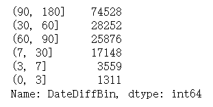
将所有的间隔时间列出来, 留存区间分别取（0,3]，（3,7], (7,30] , (30,60], (60,90], (90,180]

day_bins = [0,3,7,30,60,90,180]
group_customer_retent['DateDiffBin'] = pd.cut(group_customer_retent.Datediff,bins = day_bins)
group_customer_retent['DateDiffBin'].value_counts()

创建数据透视表，将用户ID作为Index

 customer_rent=pd.pivot_table(group_customer_retent,index='CustomerID',columns ='DateDiffBin',values=['SumPrice'],aggfunc='sum')
customer_rent.shape

customer_rent=customer_rent.applymap(lambda x:1 if x>0 else 0)
(customer_rent.sum()/customer_rent.shape[0]).plot.bar()
plt.grid()
plt.show()

(customer_rent.sum()/customer_rent.shape[0])

只有3.2%在第一次消费的次日至3天内有过消费，6.6%的客户在4-7天有过消费。分别有40.5%和37.4%的客户在首次消费后的第二个月内和第三个月内有过购买行为。将时间范围继续放宽，有高达67%的客户在90天至半年内消费过。说明该电商网站的客户群体，其采购并非高频行为，但留存下来的老客户忠诚度却极高。结合前文，仅有首次购买行为的客户占总客户的37.5%，如能提高这部分群体的留存率，将会带来很高的收益

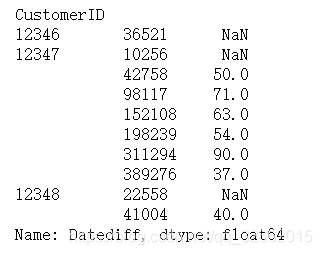
购买周期

group_customer_retent.head()

buy_cycle =group_customer_retent.drop('DateDiffBin',axis=1)

def diff(group):
    d= group.Datediff-group.Datediff.shift(1)
    return d
buy_cycle.drop_duplicates(subset=['CustomerID','Date'],keep='first',inplace=True)
buy_cycle.sort_values(by='Date',ascending=True)
uy_cycle=buy_cycle.groupby('CustomerID').apply(diff)
buy_cycle.head(10)

shift 函数应用，shift（1）数据下移动一行

buy_cycle.hist(bins=70,figsize=(12,6))
plt.xlabel(r'days')
plt.ylabel(r'frequency')
plt.show()

一个右偏分布，峰值在20-70天，说明大部分留存客户的购买周期集中于此,建议可以每隔30天左右对客户进行些优惠活动的信息推送,比较符合大部分购买周期

5.RFM模型

R：最近购买的时间
F：购买的频次
M：购买的总金额

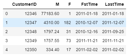
RMF_data =df_cust_action.groupby('CustomerID').agg({'SumPrice':'sum','InvoiceNo':'count','Date':['min','max']})
RMF_data=RMF_data.reset_index()
RMF_data.columns=['CustomerID','M','F','FstTime','LastTime']
RMF_data.head()

定义函数，获取R

from math import ceil
def func(data):
    R=[]
    NowTime = pd.to_datetime('2011-12-10',format='%Y-%m-%d')
    diff_R = (NowTime-data.LastTime).dt.days
    for i in diff_R:
        R.append(i)
    np.array(R)
    return R

将R加入数据中

R=func(RMF_data)
R =pd.DataFrame(R,columns=['R'])
RMF_data=pd.concat([RMF_data,R],axis=1)
RMF_data.drop(['FstTime','LastTime'],axis=1,inplace=True)
RMF_data.describe()

分别观察R,M,F的图像

fig =plt.figure(figsize=(10,12))
plt.subplot(3,1,1)
sns.distplot(RMF_data.M,label='Money')
plt.subplot(3,1,2)
plt.subplots_adjust(hspace=0.3)
sns.distplot(RMF_data.F,label='Frequency')
plt.subplot(3,1,3)
sns.distplot(RMF_data.R,label='Recency')
plt.show()

用对数函数对目标数据进行转换：目的（1）变换后可以更便捷发现数据的关系 （2）数据有偏，可以拉开数据差异 （3）数据模型符合理论模型的假设，取对数后性质和相关关系不会改变，但压缩了尺度，方便计算。

from scipy.special import boxcox,inv_boxcox
columns=['R','M','F']
for i in columns:
     RMF_data[i]=boxcox(RMF_data[i],0)

fig =plt.figure(figsize=(10,12))
plt.subplot(3,1,1)
sns.distplot(RMF_data.M,label='Money')
plt.subplot(3,1,2)
plt.subplots_adjust(hspace=0.3)
sns.distplot(RMF_data.F,label='Frequency')
plt.subplot(3,1,3)
sns.distplot(RMF_data.R,label='Recency')
plt.show()

sklearn库，数据的标准化

from sklearn.preprocessing import StandardScaler
from sklearn.cluster import KMeans
X=RMF_data.iloc[:,1:]
std_scaler =StandardScaler()
X_std =std_scaler.fit_transform(X)

kmeans ，确定K值，‘肘点法’，随着K的增大，每个样本的划分会更加精细，SSE（误差平方和会逐渐减小）。当k小于真实聚类数时，由于k的增大会大幅增加每个簇的聚合程度，故SSE的下降幅度会很大，而当k到达真实聚类数时，再增加k所得到的聚合程度回报会迅速变小，所以SSE的下降幅度会骤减，然后随着k值的继续增大而趋于平缓，也就是说SSE和k的关系图是一个手肘的形状，而这个肘部对应的k值就是数据的真实聚类数

ks = range(1,9)
inertias=[]
for k in ks :
    kc = KMeans(n_clusters=k,random_state=1)
    kc.fit(X_std)
    inertias.append(kc.inertia_)
    fig =plt.figure(figsize=(8,6))
    
plt.plot(ks, inertias, '-o')
plt.xlabel('Number of clusters, k')
plt.ylabel('Inertia')
plt.title('What is the Best Number for KMeans ?')
plt.show()

由图中可以看出，当K为2,3时，损失函数下降最快，考虑到分2类的意义不大，因此选择K=3

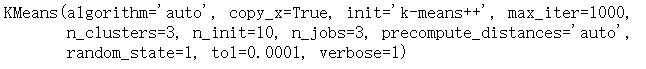
kmeans=KMeans(n_clusters=3,random_state=1,n_jobs=3,verbose=1,max_iter=1000)
kmeans.fit(X_std)

将kmeans.labels_标签添加

RMF_data =pd.concat([RMF_data,pd.DataFrame(kmeans.labels_,columns=['Label'])],axis=1)

columns=['R','M','F']
for i in columns:
     RMF_data[i]=inv_boxcox(RMF_data[i],0)
     RMF_data.CustomerID=RMF_data.CustomerID.astype(str)

查看各个标签的数据

RMF_data.groupby(['Label']).mean()
RMF_data.Label.value_counts()

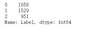
可以看出类别2的R,M,F都很高，属于重要价值客户，或者VIP用户，可以对类别02的用户群体采取重点跟进维系措施