Assignment | 01-week3 -Planar data classification with one hidden layer

该系列仅在原课程基础上课后作业部分添加个人学习笔记，或相关推导补充等。如有错误，还请批评指教。在学习了 Andrew Ng 课程的基础上，为了更方便的查阅复习，将其整理成文字。因本人一直在学习英语，所以该系列以英文为主，同时也建议读者以英文为主，中文辅助，以便后期进阶时，为学习相关领域的学术论文做铺垫。- ZJ

Coursera 课程 |deeplearning.ai |网易云课堂

---

转载请注明作者和出处：ZJ 微信公众号-「SelfImprovementLab」

知乎：https://zhuanlan.zhihu.com/c_147249273

CSDN：http://blog.csdn.net/junjun_zhao/article/details/79005099

---

一个 hidden layer 二维数据分类

Welcome to your week 3 programming assignment. It’s time to build your first neural network, which will have a hidden layer. You will see a big difference between this model and the one you implemented using logistic regression.

You will learn how to:
- Implement a 2-class classification neural network with a single hidden layer 实现二分类NN
- Use units with a non-linear activation function, such as tanh 使用 tanh 非线性激活函数
- Compute the cross entropy loss 计算交叉熵损失
- Implement forward and backward propagation 实现正向反向传播

1 - Packages

Let’s first import all the packages that you will need during this assignment.
- numpy is the fundamental package for scientific computing with Python.
- sklearn provides simple and efficient tools for data mining and data analysis. 对数据挖掘和数据分析提供简单有效的工具
- matplotlib is a library for plotting graphs in Python.
- testCases provides some test examples to assess the correctness of your functions 检查函数的正确性
- planar_utils provide various useful functions used in this assignment

# Package imports
import numpy as np
import matplotlib.pyplot as plt
from testCases_v2 import *
import sklearn
import sklearn.datasets
import sklearn.linear_model
from planar_utils import plot_decision_boundary, sigmoid, load_planar_dataset, load_extra_datasets

%matplotlib inline

np.random.seed(1) # set a seed so that the results are consistent 结果是一致的 是随机结果是可预测的

/opt/conda/lib/python3.5/site-packages/matplotlib/font_manager.py:273: UserWarning: Matplotlib is building the font cache using fc-list. This may take a moment.
  warnings.warn('Matplotlib is building the font cache using fc-list. This may take a moment.')
/opt/conda/lib/python3.5/site-packages/matplotlib/font_manager.py:273: UserWarning: Matplotlib is building the font cache using fc-list. This may take a moment.
  warnings.warn('Matplotlib is building the font cache using fc-list. This may take a moment.')

# 使结果是可预测的
np.random.seed(0)
A= np.random.rand(4)
print(A)
# array([ 0.55,  0.72,  0.6 ,  0.54])
np.random.seed(0)
B = np.random.rand(4)
print(B)
# array([ 0.55,  0.72,  0.6 ,  0.54])
# [ 0.5488135   0.71518937  0.60276338  0.54488318]
# [ 0.5488135   0.71518937  0.60276338  0.54488318]

[ 0.5488135   0.71518937  0.60276338  0.54488318]
[ 0.5488135   0.71518937  0.60276338  0.54488318]

2 - Dataset

First, let’s get the dataset you will work on. 获取将要用到的数据集，The following code will load a “flower” 2-class dataset into variables X and Y. 加载 flower 的二分类数据

X, Y = load_planar_dataset()

Visualize the dataset using matplotlib. 使用 matplotlib 可视化数据 The data looks like a “flower” with some red (label y=0) and some blue (y=1) points. Your goal is to build a model to fit this data. 目标是建立一个符合这个数据的模型

# Visualize the data:
# X[0, :] X 中 0 行左右列  
plt.scatter(X[0, :], X[1, :], c=Y, s=40, cmap=plt.cm.Spectral);
# 下图是一朵花 由红色和蓝色的点组成

You have:
- a numpy-array (matrix) X that contains your features (x1, x2) X 特征
- a numpy-array (vector) Y that contains your labels (red:0, blue:1). Y 标签 red or blue

Lets first get a better sense of what our data is like.

Exercise: How many training examples do you have? In addition, what is the shape of the variables X and Y?

Hint: How do you get the shape of a numpy array? (help)

### START CODE HERE ### (≈ 3 lines of code)
shape_X = X.shape
shape_Y = Y.shape
m = X.shape[1]  # training set size X.shape[1] (n,m) n 是单个训练样本的特征 m 是 训练样本总量
### END CODE HERE ###

print ('The shape of X is: ' + str(shape_X))
print ('The shape of Y is: ' + str(shape_Y))
print ('I have m = %d training examples!' % (m))

The shape of X is: (2, 400)
The shape of Y is: (1, 400)
I have m = 400 training examples!

Expected Output:

shape of X	(2, 400)
shape of Y	(1, 400)
m	400

3 - Simple Logistic Regression

Before building a full neural network, lets first see how logistic regression performs on this problem. You can use sklearn’s built-in functions to do that. Run the code below to train a logistic regression classifier on the dataset.

# Train the logistic regression classifier 训练  logistic 回归 分类
# clf = sklearn.linear_model.LogisticRegressionCV();
# clf.fit(X.T, Y.T);

clf = sklearn.linear_model.LogisticRegressionCV()
# X is: (2, 400)   Y is: (1, 400) X.T (400,2) Y.T(400,1)
clf.fit(X.T,Y.T)

/opt/conda/lib/python3.5/site-packages/sklearn/utils/validation.py:515: DataConversionWarning: A column-vector y was passed when a 1d array was expected. Please change the shape of y to (n_samples, ), for example using ravel().
  y = column_or_1d(y, warn=True)





LogisticRegressionCV(Cs=10, class_weight=None, cv=None, dual=False,
           fit_intercept=True, intercept_scaling=1.0, max_iter=100,
           multi_class='ovr', n_jobs=1, penalty='l2', random_state=None,
           refit=True, scoring=None, solver='lbfgs', tol=0.0001, verbose=0)

You can now plot the decision boundary of these models. Run the code below.

# Plot the decision boundary for logistic regression 画分界线 决策边界
# plot_decision_boundary(lambda x: clf.predict(x), X, Y)
# plt.title("Logistic Regression")

plot_decision_boundary(lambda x: clf.predict(x), X, Y)
plt.title('Logistic Regression')

# Print accuracy 打印精度，上面的 cell 是训练数据 这里是 预测 predict 数据 LR_predictions 相当于 yhat 预测值
LR_predictions = clf.predict(X.T)
# 
print ('Accuracy of logistic regression: %d ' % float((np.dot(Y,LR_predictions) + np.dot(1-Y,1-LR_predictions))/float(Y.size)*100) +
       '% ' + "(percentage of correctly labelled datapoints)")
# 下图所示 logistic 回归 对线性可分的数据处理是 画一条线 下图红色 和蓝色背景是进行的分类，很显然 数据不是线性可分的 所以 效果不好 正确率很低

Accuracy of logistic regression: 47 % (percentage of correctly labelled datapoints)

Expected Output:

Accuracy

47%

Interpretation: The dataset is not linearly separable, 这个数据集不是线性可分的，所以 logistic 回归效果并不好 so logistic regression doesn’t perform well. Hopefully a neural network will do better. Let’s try this now! 来试一试 神经网络怎么样

4 - Neural Network model

Logistic regression did not work well on the “flower dataset”. You are going to train a Neural Network with a single hidden layer.

Here is our model:

Mathematically:

For one example x(i) x ( i ) :

z[1](i)=W[1]x(i)+b[1](i)(1) (1) z [ 1 ] ( i ) = W [ 1 ] x ( i ) + b [ 1 ] ( i )

a[1](i)=tanh(z[1](i))(2) (2) a [ 1 ] ( i ) = tanh ⁡ ( z [ 1 ] ( i ) )

z[2](i)=W[2]a[1](i)+b[2](i)(3) (3) z [ 2 ] ( i ) = W [ 2 ] a [ 1 ] ( i ) + b [ 2 ] ( i )

ŷ (i)=a[2](i)=σ(z[2](i))(4) (4) y ^ ( i ) = a [ 2 ] ( i ) = σ ( z [ 2 ] ( i ) )

y(i)prediction={10if a[2](i)>0.5otherwise (5) (5) y p r e d i c t i o n ( i ) = { 1 if  a [ 2 ] ( i ) > 0.5 0 otherwise 

Given the predictions on all the examples, you can also compute the cost J J as follows:

J=−1m∑i=0m(y(i)log(a[2](i))+(1−y(i))log(1−a[2](i)))(6) (6) J = − 1 m ∑ i = 0 m ( y ( i ) log ⁡ ( a [ 2 ] ( i ) ) + ( 1 − y ( i ) ) log ⁡ ( 1 − a [ 2 ] ( i ) ) )

Reminder: The general methodology to build a Neural Network is to:
1. Define the neural network structure ( # of input units, # of hidden units, etc).
2. Initialize the model’s parameters
3. Loop:
- Implement forward propagation
- Compute loss
- Implement backward propagation to get the gradients
- Update parameters (gradient descent)

You often build helper functions to compute steps 1-3 and then merge them into one function we call nn_model(). Once you’ve built nn_model() and learnt the right parameters, you can make predictions on new data. 创建1-3 的辅助函数然后将他们合并到 nn_model() 中，一旦你创建了 nn_model() 然后学习到了正确的参数，就可以使用的新的数据做预测。

4.1 - Defining the neural network structure

定义神经网络结构

Exercise: Define three variables:
- n_x: the size of the input layer 输入层大小
- n_h: the size of the hidden layer (set this to 4) 隐含层大小
- n_y: the size of the output layer 输出层大小

Hint: Use shapes of X and Y to find n_x and n_y. Also, hard code the hidden layer size to be 4.
利用 X Y ‘s shape 去找到 n_x and n_y ，硬编码 使 hidden 层为4

由上面我们可以总结出，在神经网络中，我们以相邻两层为观测对象，前面一层作为输入，后面一层作为输出，两层之间的w参数矩阵大小为 (nout,nin) ( n o u t , n i n ) ，b参数矩阵大小为 (nout,1) ( n o u t , 1 ) ，这里是作为 z=wX+b z = w X + b 的线性关系来说明的，在神经网络中， w[i]=wT w [ i ] = w T 。

# GRADED FUNCTION: layer_sizes

def layer_sizes(X, Y):
    """
    Arguments:
    X -- input dataset of shape (input size, number of examples)
    Y -- labels of shape (output size, number of examples)

    Returns:
    n_x -- the size of the input layer
    n_h -- the size of the hidden layer
    n_y -- the size of the output layer
    """
    ### START CODE HERE ### (≈ 3 lines of code)
    n_x = X.shape[0] # size of input layer
    n_h = 4
    n_y = Y.shape[0] # size of output layer
    # ??? why ？     
    ### END CODE HERE ###
    return (n_x, n_h, n_y)

X_assess, Y_assess = layer_sizes_test_case()
(n_x, n_h, n_y) = layer_sizes(X_assess, Y_assess)
print("The size of the input layer is: n_x = " + str(n_x))
print("The size of the hidden layer is: n_h = " + str(n_h))
print("The size of the output layer is: n_y = " + str(n_y))

The size of the input layer is: n_x = 5
The size of the hidden layer is: n_h = 4
The size of the output layer is: n_y = 2

Expected Output (these are not the sizes you will use for your network, they are just used to assess the function you’ve just coded).

n_x	5
n_h	4
n_y	2

4.2 - Initialize the model’s parameters

Exercise: Implement the function initialize_parameters().

Instructions:
- Make sure your parameters’ sizes are right. Refer to the neural network figure above if needed.
- You will initialize the weights matrices （W 系数权重）with random values.
- Use: np.random.randn(a,b) * 0.01 to randomly initialize a matrix of shape (a,b).
- You will initialize the bias vectors (b-偏移量) as zeros.
- Use: np.zeros((a,b)) to initialize a matrix of shape (a,b) with zeros.

由上面我们可以总结出，在神经网络中，我们以相邻两层为观测对象，前面一层作为输入，后面一层作为输出，两层之间的w参数矩阵大小为 (nout,nin) ( n o u t , n i n ) ，b参数矩阵大小为 (nout,1) ( n o u t , 1 ) ，这里是作为 z=wX+b z = w X + b 的线性关系来说明的，在神经网络中， w[i]=wT w [ i ] = w T 。

# GRADED FUNCTION: initialize_parameters

def initialize_parameters(n_x, n_h, n_y):
    """
    Argument:
    n_x -- size of the input layer
    n_h -- size of the hidden layer
    n_y -- size of the output layer

    Returns:
    params -- python dictionary containing your parameters:
                    W1 -- weight matrix of shape (n_h, n_x)
                    b1 -- bias vector of shape (n_h, 1)
                    W2 -- weight matrix of shape (n_y, n_h)
                    b2 -- bias vector of shape (n_y, 1)
    """

    np.random.seed(2) # we set up a seed so that your output matches ours although the initialization is random.

    ### START CODE HERE ### (≈ 4 lines of code)
    W1 = np.random.randn(n_h,n_x)
    b1 = np.zeros((n_h,1))
    W2 = np.random.randn(n_y,n_h)
    b2 = np.zeros((n_y,1))
    ### END CODE HERE ###

    assert (W1.shape == (n_h, n_x))
    assert (b1.shape == (n_h, 1))
    assert (W2.shape == (n_y, n_h))
    assert (b2.shape == (n_y, 1))

    parameters = {"W1": W1,
                  "b1": b1,
                  "W2": W2,
                  "b2": b2}

    return parameters

n_x, n_h, n_y = initialize_parameters_test_case()

parameters = initialize_parameters(n_x, n_h, n_y)
print("W1 = \n" + str(parameters["W1"]))
print("b1 = \n" + str(parameters["b1"]))
print("W2 = " + str(parameters["W2"]))
print("b2 = " + str(parameters["b2"]))

W1 = 
[[-0.41675785 -0.05626683]
 [-2.1361961   1.64027081]
 [-1.79343559 -0.84174737]
 [ 0.50288142 -1.24528809]]
b1 = 
[[ 0.]
 [ 0.]
 [ 0.]
 [ 0.]]
W2 = [[-1.05795222 -0.90900761  0.55145404  2.29220801]]
b2 = [[ 0.]]

Expected Output:

W1	[[-0.00416758 -0.00056267] [-0.02136196 0.01640271] [-0.01793436 -0.00841747] [ 0.00502881 -0.01245288]]
b1	[[ 0.] [ 0.] [ 0.] [ 0.]]
W2	[[-0.01057952 -0.00909008 0.00551454 0.02292208]]
b2	[[ 0.]]

4.3 - The Loop

Question: Implement forward_propagation().

Instructions:
- Look above at the mathematical representation of your classifier. 看上面用于分类的数学表达式
- You can use the function sigmoid(). It is built-in (imported) in the notebook.
- You can use the function np.tanh(). It is part of the numpy library.
- The steps you have to implement are:
1. Retrieve each parameter from the dictionary “parameters” (which is the output of initialize_parameters()) by using parameters[".."].
2. Implement Forward Propagation. Compute Z[1],A[1],Z[2] Z [ 1 ] , A [ 1 ] , Z [ 2 ] and A[2] A [ 2 ] (the vector of all your predictions on all the examples in the training set).
- Values needed in the backpropagation are stored in “cache“. The cache will be given as an input to the backpropagation function.

# GRADED FUNCTION: forward_propagation

def forward_propagation(X, parameters):
    """
    Argument:
    X -- input data of size (n_x, m)
    parameters -- python dictionary containing your parameters (output of initialization function)

    Returns:
    A2 -- The sigmoid output of the second activation
    cache -- a dictionary containing "Z1", "A1", "Z2" and "A2"
    """
    # Retrieve each parameter from the dictionary "parameters"
    ### START CODE HERE ### (≈ 4 lines of code)
    W1 = parameters["W1"]
    b1 = parameters["b1"]
    W2 = parameters["W2"]
    b2 = parameters["b2"]
    ### END CODE HERE ###

    # Implement Forward Propagation to calculate A2 (probabilities)
    ### START CODE HERE ### (≈ 4 lines of code)
    Z1 = np.dot(W1, X) + b1
    A1 = np.tanh(Z1)
    Z2 = np.dot(W2, A1) + b2 
    A2 = sigmoid(Z2)
    ### END CODE HERE ###

    assert(A2.shape == (1, X.shape[1]))

    cache = {"Z1": Z1,
             "A1": A1,
             "Z2": Z2,
             "A2": A2}

    return A2, cache

X_assess, parameters = forward_propagation_test_case()
A2, cache = forward_propagation(X_assess, parameters)

# Note: we use the mean here just to make sure that your output matches ours. 
print(np.mean(cache['Z1']) ,np.mean(cache['A1']),np.mean(cache['Z2']),np.mean(cache['A2']))

0.262818640198 0.091999045227 -1.30766601287 0.212877681719

Expected Output:

0.262818640198 0.091999045227 -1.30766601287 0.212877681719

Now that you have computed A[2] A [ 2 ] (in the Python variable “A2“), which contains a[2](i) a [ 2 ] ( i ) for every example, you can compute the cost function as follows:

J=−1m∑i=0m(y(i)log(a[2](i))+(1−y(i))log(1−a[2](i)))(13) (13) J = − 1 m ∑ i = 0 m ( y ( i ) log ⁡ ( a [ 2 ] ( i ) ) + ( 1 − y ( i ) ) log ⁡ ( 1 − a [ 2 ] ( i ) ) )

Exercise: Implement compute_cost() to compute the value of the cost J J .

Instructions:
- There are many ways to implement the cross-entropy loss. To help you, we give you how we would have implemented
−∑i=0my(i)log(a[2](i)) − ∑ i = 0 m y ( i ) log ⁡ ( a [ 2 ] ( i ) ) :

logprobs = np.multiply(np.log(A2),Y)
cost = - np.sum(logprobs)                # no need to use a for loop!

(you can use either np.multiply() and then np.sum() or directly np.dot()).

np.dot()- 相乘且相加

np.multiply()- 仅相乘

np.sum()-仅相加

# GRADED FUNCTION: compute_cost

def compute_cost(A2, Y, parameters):
    """
    Computes the cross-entropy cost given in equation (13)

    Arguments:
    A2 -- The sigmoid output of the second activation, of shape (1, number of examples)
    Y -- "true" labels vector of shape (1, number of examples)
    parameters -- python dictionary containing your parameters W1, b1, W2 and b2

    Returns:
    cost -- cross-entropy cost given equation (13)
    """

    m = Y.shape[1] # number of example

    # Compute the cross-entropy cost
    ### START CODE HERE ### (≈ 2 lines of code)
    logprobs = np.multiply(Y,np.log(A2))
    cost = - np.sum(logprobs)
    ### END CODE HERE ###

    cost = np.squeeze(cost)     # makes sure cost is the dimension we expect.  确保成本是我们期望维度。
                                # E.g., turns [[17]] into 17  float 
    assert(isinstance(cost, float))

    return cost

A2, Y_assess, parameters = compute_cost_test_case()

print("cost = " + str(compute_cost(A2, Y_assess, parameters)))

cost = 0.692685886972

Expected Output:

cost	0.693058761…

Using the cache computed during forward propagation, you can now implement backward propagation.
在正向传播得到的 cache,可以用来实现反向传播

Question: Implement the function backward_propagation().

Instructions:
Backpropagation is usually the hardest (most mathematical) part in deep learning. To help you, here again is the slide from the lecture on backpropagation. You’ll want to use the six equations on the right of this slide, since you are building a vectorized implementation.
反向传播通常是深度学习中最难的一部分，

• Tips:

  • To compute dZ1 you’ll need to compute g[1]′(Z[1]) g [ 1 ] ′ ( Z [ 1 ] ) . Since g[1](.) g [ 1 ] ( . ) is the tanh activation function, if a=g[1](z) a = g [ 1 ] ( z ) then g[1]′(z)=1−a2 g [ 1 ] ′ ( z ) = 1 − a 2 . So you can compute
    g[1]′(Z[1]) g [ 1 ] ′ ( Z [ 1 ] ) using (1 - np.power(A1, 2)).

  导数 a=g[1](z) a = g [ 1 ] ( z ) -> g[1]′(z)=1−a2 g [ 1 ] ′ ( z ) = 1 − a 2 g 是个函数 相当于g(z) 不是相乘 不要理解错了

# GRADED FUNCTION: backward_propagation

def backward_propagation(parameters, cache, X, Y):
    """
    Implement the backward propagation using the instructions above.

    Arguments:
    parameters -- python dictionary containing our parameters 
    cache -- a dictionary containing "Z1", "A1", "Z2" and "A2".
    X -- input data of shape (2, number of examples)
    Y -- "true" labels vector of shape (1, number of examples)

    Returns:
    grads -- python dictionary containing your gradients with respect to different parameters
    """
    #  X.shape[1] 样本总个数   
    m = X.shape[1]

    # First, retrieve W1 and W2 from the dictionary "parameters".
    ### START CODE HERE ### (≈ 2 lines of code)
    W1 = parameters["W1"]
    W2 = parameters["W2"]
    ### END CODE HERE ###

    # Retrieve also A1 and A2 from dictionary "cache".
    ### START CODE HERE ### (≈ 2 lines of code)
    A1 = cache["A1"]
    A2 = cache["A2"]
    ### END CODE HERE ###

    # Backward propagation: calculate dW1, db1, dW2, db2. 
    ### START CODE HERE ### (≈ 6 lines of code, corresponding to 6 equations on slide above)
    dZ2 = A2 - Y
    # 注意：A1.T     
    dW2 = (1.0/m)*np.dot(dZ2,A1.T)
    db2 = (1.0/m)*np.sum(dZ2,axis=1,keepdims=True)
    # 注意：W2.T  
    dZ1 = np.dot(W2.T,dZ2)*(1-np.power(A1,2))
    # 注意：X.T
    dW1 = (1.0/m)*np.dot(dZ1,X.T)
    db1 = (1.0/m)*np.sum(dZ1,axis=1,keepdims=True)
    ### END CODE HERE ###

    grads = {"dW1": dW1,
             "db1": db1,
             "dW2": dW2,
             "db2": db2}

    return grads

parameters, cache, X_assess, Y_assess = backward_propagation_test_case()

grads = backward_propagation(parameters, cache, X_assess, Y_assess)
print ("dW1 = "+ str(grads["dW1"]))
print ("db1 = "+ str(grads["db1"]))
print ("dW2 = "+ str(grads["dW2"]))
print ("db2 = "+ str(grads["db2"]))

dW1 = [[ 0.00301023 -0.00747267]
 [ 0.00257968 -0.00641288]
 [-0.00156892  0.003893  ]
 [-0.00652037  0.01618243]]
db1 = [[ 0.00176201]
 [ 0.00150995]
 [-0.00091736]
 [-0.00381422]]
dW2 = [[ 0.00078841  0.01765429 -0.00084166 -0.01022527]]
db2 = [[-0.16655712]]

Expected output:

dW1	[[ 0.00301023 -0.00747267] [ 0.00257968 -0.00641288] [-0.00156892 0.003893 ] [-0.00652037 0.01618243]]
db1	[[ 0.00176201] [ 0.00150995] [-0.00091736] [-0.00381422]]
dW2	[[ 0.00078841 0.01765429 -0.00084166 -0.01022527]]
db2	[[-0.16655712]]

Question: Implement the update rule. Use gradient descent. You have to use (dW1, db1, dW2, db2) in order to update (W1, b1, W2, b2).

General gradient descent rule: θ=θ−α∂J∂θ θ = θ − α ∂ J ∂ θ where α α is the learning rate and θ θ represents a parameter.

Illustration: The gradient descent algorithm with a good learning rate (converging)一个好的学习速率会收敛 and a bad learning rate (diverging).一个坏的学习速率会发散 Images courtesy of Adam Harley.

# GRADED FUNCTION: update_parameters

def update_parameters(parameters, grads, learning_rate = 1.2):
    """
    Updates parameters using the gradient descent update rule given above

    Arguments:
    parameters -- python dictionary containing your parameters 
    grads -- python dictionary containing your gradients 

    Returns:
    parameters -- python dictionary containing your updated parameters 
    """
    # Retrieve each parameter from the dictionary "parameters"
    ### START CODE HERE ### (≈ 4 lines of code)
    W1 = parameters["W1"]
    b1 = parameters["b1"]
    W2 = parameters["W2"]
    b2 = parameters["b2"]
    ### END CODE HERE ###

    # Retrieve each gradient from the dictionary "grads"
    ### START CODE HERE ### (≈ 4 lines of code)
    dW1 = grads["dW1"]
    db1 = grads["db1"]
    dW2 = grads["dW2"]
    db2 = grads["db2"]
    ## END CODE HERE ###

    # Update rule for each parameter
    ### START CODE HERE ### (≈ 4 lines of code)
    W1 = W1 - learning_rate*dW1
    b1 = b1 - learning_rate*db1
    W2 = W2 - learning_rate*dW2
    b2 = b2 - learning_rate*db2
    ### END CODE HERE ###

    parameters = {"W1": W1,
                  "b1": b1,
                  "W2": W2,
                  "b2": b2}

    return parameters

parameters, grads = update_parameters_test_case()
parameters = update_parameters(parameters, grads)

print("W1 = \n" + str(parameters["W1"]))
print("b1 = \n " + str(parameters["b1"]))
print("W2 = " + str(parameters["W2"]))
print("b2 = " + str(parameters["b2"]))

W1 = 
[[-0.00643025  0.01936718]
 [-0.02410458  0.03978052]
 [-0.01653973 -0.02096177]
 [ 0.01046864 -0.05990141]]
b1 = 
 [[ -1.02420756e-06]
 [  1.27373948e-05]
 [  8.32996807e-07]
 [ -3.20136836e-06]]
W2 = [[-0.01041081 -0.04463285  0.01758031  0.04747113]]
b2 = [[ 0.00010457]]

Expected Output:

W1	[[-0.00643025 0.01936718] [-0.02410458 0.03978052] [-0.01653973 -0.02096177] [ 0.01046864 -0.05990141]]
b1	[[ -1.02420756e-06] [ 1.27373948e-05] [ 8.32996807e-07] [ -3.20136836e-06]]
W2	[[-0.01041081 -0.04463285 0.01758031 0.04747113]]
b2	[[ 0.00010457]]

4.4 - Integrate parts 4.1, 4.2 and 4.3 in nn_model()

集成合并上面的辅助函数 到 nn_model()

Question: Build your neural network model in nn_model().

Instructions: The neural network model has to use the previous functions in the right order.

# GRADED FUNCTION: nn_model

def nn_model(X, Y, n_h, num_iterations = 10000, print_cost=False):
    """
    Arguments:
    X -- dataset of shape (2, number of examples)
    Y -- labels of shape (1, number of examples)
    n_h -- size of the hidden layer
    num_iterations -- Number of iterations in gradient descent loop
    print_cost -- if True, print the cost every 1000 iterations

    Returns:
    parameters -- parameters learnt by the model. They can then be used to predict.
    """

    np.random.seed(3)
    #  layer_sizes 返回三个参数 ，索引对应取值
    n_x = layer_sizes(X, Y)[0]
    n_y = layer_sizes(X, Y)[2]

    # Initialize parameters, then retrieve W1, b1, W2, b2. Inputs: "n_x, n_h, n_y". Outputs = "W1, b1, W2, b2, parameters".
    ### START CODE HERE ### (≈ 5 lines of code)
    parameters = initialize_parameters(n_x, n_h, n_y)
    W1 = parameters["W1"]
    b1 = parameters["b1"]
    W2 = parameters["W2"]
    b2 = parameters["b2"]
    ### END CODE HERE ###

    # Loop (gradient descent)

    for i in range(0, num_iterations):

        ### START CODE HERE ### (≈ 4 lines of code)
        # Forward propagation. Inputs: "X, parameters". Outputs: "A2, cache". 
        A2, cache = forward_propagation(X, parameters)

        # Cost function. Inputs: "A2, Y, parameters". Outputs: "cost".
        cost = compute_cost(A2, Y, parameters)

        # Backpropagation. Inputs: "parameters, cache, X, Y". Outputs: "grads".
        grads = backward_propagation(parameters, cache, X, Y)

        # Gradient descent parameter update. Inputs: "parameters, grads". Outputs: "parameters".
        parameters = update_parameters(parameters, grads)


        # 1.正向传播 2.计算 cost 3.反向传播 4. 更新参数
        ### END CODE HERE ###

        # Print the cost every 1000 iterations
        if print_cost and i % 1000 == 0:
            print ("Cost after iteration %i: %f" %(i, cost))

    return parameters

X_assess, Y_assess = nn_model_test_case()
parameters = nn_model(X_assess, Y_assess, 4, num_iterations=10000, print_cost=True)
print("W1 = " + str(parameters["W1"]))
print("b1 = " + str(parameters["b1"]))
print("W2 = " + str(parameters["W2"]))
print("b2 = " + str(parameters["b2"]))

Cost after iteration 0: 0.074560
Cost after iteration 1000: 0.000439
Cost after iteration 2000: 0.000222
Cost after iteration 3000: 0.000148
Cost after iteration 4000: 0.000111
Cost after iteration 5000: 0.000089
Cost after iteration 6000: 0.000074
Cost after iteration 7000: 0.000064
Cost after iteration 8000: 0.000056
Cost after iteration 9000: 0.000050
W1 = [[-0.89587042  1.18044635]
 [-2.14783312  1.70666862]
 [-1.50260821 -1.21347886]
 [ 0.80826745 -1.65434514]]
b1 = [[ 0.19050922]
 [ 0.01614166]
 [-0.34103273]
 [-0.25208981]]
W2 = [[-2.90757381 -3.18177289  0.36186225  4.50758023]]
b2 = [[ 0.24451252]]

Expected Output:

cost after iteration 0	0.692739
⋮ ⋮	⋮ ⋮
W1	[[-0.65848169 1.21866811] [-0.76204273 1.39377573] [ 0.5792005 -1.10397703] [ 0.76773391 -1.41477129]]
b1	[[ 0.287592 ] [ 0.3511264 ] [-0.2431246 ] [-0.35772805]]
W2	[[-2.45566237 -3.27042274 2.00784958 3.36773273]]
b2	[[ 0.20459656]]

4.5 Predictions

Question: Use your model to predict by building predict().
Use forward propagation to predict results. 最后 使用 正向传播预测结果

Reminder: predictions = yprediction=?{activation > 0.5}={10if activation>0.5otherwise y p r e d i c t i o n = 1 {activation > 0.5} = { 1 if   a c t i v a t i o n > 0.5 0 otherwise

As an example, if you would like to set the entries of a matrix X to 0 and 1 based on a threshold you would do: X_new = (X > threshold)
介绍一个方法，如果你希望 设置 一个矩阵X 的元素 是 0 或 1 基于一个阈值

# GRADED FUNCTION: predict

def predict(parameters, X):
    """
    Using the learned parameters, predicts a class for each example in X

    Arguments:
    parameters -- python dictionary containing your parameters 
    X -- input data of size (n_x, m)

    Returns
    predictions -- vector of predictions of our model (red: 0 / blue: 1)
    """

    # Computes probabilities using forward propagation, and classifies to 0/1 using 0.5 as the threshold.
    ### START CODE HERE ### (≈ 2 lines of code)
    # X 原始训练集 和最后 更新学习过后的参数    
    A2, cache = forward_propagation(X, parameters)
    predictions = (A2 > 0.5)
    print('predictions:',predictions.shape)        
    ### END CODE HERE ###

    return predictions

parameters, X_assess = predict_test_case()

predictions = predict(parameters, X_assess)
print("predictions mean = " + str(np.mean(predictions)))

predictions: (1, 3)
predictions mean = 0.666666666667

Expected Output:

predictions mean

0.666666666667

It is time to run the model and see how it performs on a planar dataset. Run the following code to test your model with a single hidden layer of nh n h hidden units.

# Build a model with a n_h-dimensional hidden layer
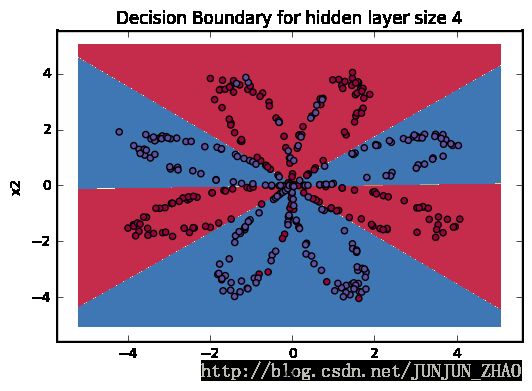
parameters = nn_model(X, Y, n_h = 4, num_iterations = 10000, print_cost=True)

# Plot the decision boundary 
plot_decision_boundary(lambda x: predict(parameters, x.T), X, Y)
plt.title("Decision Boundary for hidden layer size " + str(4))
# 如下图所示，非线性可分 使用 一层的NN 很好的 进行了划分

Cost after iteration 0: 236.669141
Cost after iteration 1000: 57.670439
Cost after iteration 2000: 55.153507
Cost after iteration 3000: 53.523063
Cost after iteration 4000: 52.503785
Cost after iteration 5000: 51.767575
Cost after iteration 6000: 51.208205
Cost after iteration 7000: 50.768882
Cost after iteration 8000: 50.414702
Cost after iteration 9000: 50.122855
predictions: (1, 1038240)

Expected Output:

Cost after iteration 9000

0.218607

# Print accuracy
predictions = predict(parameters, X)
print ('Accuracy: %d' % float((np.dot(Y,predictions.T) + np.dot(1-Y,1-predictions.T))/float(Y.size)*100) + '%')

predictions: (1, 400)
Accuracy: 91%

Expected Output:

Accuracy

90%

Accuracy is really high compared to Logistic Regression. The model has learnt the leaf patterns of the flower! Neural networks are able to learn even highly non-linear decision boundaries,高度非线性 决策边界 unlike logistic regression.

Now, let’s try out several hidden layer sizes.

4.6 - Tuning hidden layer size (optional/ungraded exercise)

Run the following code. It may take 1-2 minutes. You will observe different behaviors of the model for various hidden layer sizes.

# This may take about 2 minutes to run

plt.figure(figsize=(16, 32))
# 隐藏层大小取值 [1, 2, 3, 4, 5, 20, 50]
hidden_layer_sizes = [1, 2, 3, 4, 5, 20, 50]
# enumerate(hidden_layer_sizes) 迭代取值
for i, n_h in enumerate(hidden_layer_sizes):
    plt.subplot(5, 2, i+1)
    plt.title('Hidden Layer of size %d' % n_h)
    parameters = nn_model(X, Y, n_h, num_iterations = 5000)
    plot_decision_boundary(lambda x: predict(parameters, x.T), X, Y)
    predictions = predict(parameters, X)
    #     
    accuracy = float((np.dot(Y,predictions.T) + np.dot(1-Y,1-predictions.T))/float(Y.size)*100)
    print ("Accuracy for {} hidden units: {} %".format(n_h, accuracy))

predictions: (1, 1038240)
predictions: (1, 400)
Accuracy for 1 hidden units: 61.5 %
predictions: (1, 1038240)
predictions: (1, 400)
Accuracy for 2 hidden units: 70.5 %
predictions: (1, 1038240)
predictions: (1, 400)
Accuracy for 3 hidden units: 66.25 %
predictions: (1, 1038240)
predictions: (1, 400)
Accuracy for 4 hidden units: 90.75 %
predictions: (1, 1038240)
predictions: (1, 400)
Accuracy for 5 hidden units: 91.0 %
predictions: (1, 1038240)
predictions: (1, 400)
Accuracy for 20 hidden units: 91.5 %
predictions: (1, 1038240)
predictions: (1, 400)
Accuracy for 50 hidden units: 90.75 %

Interpretation:解释
- The larger models (with more hidden units) 更大的模型包含更多的隐藏单元 可以更好的匹配训练数据are able to fit the training set better, until eventually the largest models overfit the data. 直到最终 过大的模型过拟合数据
- The best hidden layer size seems to be around n_h = 5. Indeed, a value around here seems to fits the data well without also incurring noticable overfitting.没有引起明显的过拟合
- You will also learn later about regularization, 正则化 which lets you use very large models (such as n_h = 50) without much overfitting.

Optional questions:

Note: Remember to submit the assignment but clicking the blue “Submit Assignment” button at the upper-right.

Some optional/ungraded questions that you can explore if you wish:
- What happens when you change the tanh activation for a sigmoid activation or a ReLU activation?
- Play with the learning_rate. What happens?
- What if we change the dataset? (See part 5 below!)

You’ve learnt to:
- Build a complete neural network with a hidden layer
- Make a good use of a non-linear unit 使用非线性单元
- Implemented forward propagation and backpropagation, and trained a neural network
- See the impact of varying the hidden layer size, including overfitting.

Nice work!

5) Performance on other datasets

If you want, you can rerun the whole notebook (minus the dataset part) for each of the following datasets.

# Datasets
noisy_circles, noisy_moons, blobs, gaussian_quantiles, no_structure = load_extra_datasets()

datasets = {"noisy_circles": noisy_circles,
            "noisy_moons": noisy_moons,
            "blobs": blobs,
            "gaussian_quantiles": gaussian_quantiles}

### START CODE HERE ### (choose your dataset)
dataset = "noisy_moons"
### END CODE HERE ###

X, Y = datasets[dataset]
X, Y = X.T, Y.reshape(1, Y.shape[0])

# make blobs binary
if dataset == "blobs":
    Y = Y%2

# Visualize the data
plt.scatter(X[0, :], X[1, :], c=Y, s=40, cmap=plt.cm.Spectral);

Congrats on finishing this Programming Assignment!

Reference:
- http://scs.ryerson.ca/~aharley/neural-networks/
- http://cs231n.github.io/neural-networks-case-study/

---

PS: 欢迎扫码关注公众号：「SelfImprovementLab」！专注「深度学习」，「机器学习」，「人工智能」。以及 「早起」，「阅读」，「运动」，「英语 」「其他」不定期建群 打卡互助活动。