SQL Server中的数据分析表达式(DAX)入门
介绍 (Introduction)
In our SQLShack discussions over the past few weeks, we have dealt with a few of the more conventional SQL Server data manipulation techniques. Today we are going to be a bit more avant-garde and touch upon a subject dear to my heart.
在过去几周SQLShack讨论中,我们讨论了一些更常规SQL Server数据操作技术。 今天,我们将变得更加前卫,并触及我心爱的主题。
With Power Bi becoming more and more important on the business side within major industries worldwide, it is not surprising that sooner or later every SQL programmer is going to have to learn and be able to ‘talk’ DAX.
随着Power Bi在全球主要行业中的业务方面变得越来越重要,每位SQL程序员迟早都必须学习并能够“交谈” DAX不足为奇。
In this article we are going to have a look at the a few of the more important ‘constructs’ and produce production grade queries for data extraction and for reports; enabling the reader to ‘hit the ground running’.
在本文中,我们将介绍一些更重要的“结构”,并为数据提取和报告生成生产级查询。 使读者能够“踏上第一步”。
Microsoft商业智能语义模型(BISM) (The Microsoft Business Intelligence Semantic Model (BISM))
Prior to any discussion pertaining to Data Analysis Expressions or DAX, it is imperative to understand that DAX is closely link to the Business Intelligence Semantic Model (hence forward referred to as the BISM). Microsoft describes the BISM as “a single model that serves all of the end-user experiences for Microsoft BI, including reporting analysis and dash boarding”.
在进行任何有关数据分析表达式或DAX的讨论之前,必须了解DAX与商业智能语义模型(因此称为BISM)紧密相关。 微软将BISM描述为“一个为Microsoft BI提供所有最终用户体验的单一模型,包括报告分析和仪表板”。
In fact, in order to extract data from any tabular Analysis Services projects, the DAX language is the recommended language of choice. DAX itself is a rich library of expressions, functions that are used extensively within Microsoft Power Pivot and SQL Server Analysis Services tabular models. It is a ‘build out’ of Multi-Dimensional Expressions (MDX) and it does provide exciting new possibilities.
实际上,为了从任何表格形式的Analysis Services项目中提取数据,推荐使用DAX语言。 DAX本身是一个丰富的表达式库,这些函数在Microsoft Power Pivot和SQL Server Analysis Services表格模型中广泛使用。 它是多维表达式(MDX)的“构建”,确实提供了令人兴奋的新可能性。
This said let us get started.
这就是说让我们开始吧。
安装SQL Server Analysis Services的表格实例 (Installation of a Tabular Instance of SQL Server Analysis Services)
With the advent of SQL Server 2012 and up, there are two flavors of Analysis Services:
随着SQL Server 2012及更高版本的到来,Analysis Services有两种形式:
- The Multidimensional Model 多维模型
- The Tabular Model 表格模型
Both of these models require separate instances. More often than not, for any project, I normally create a relational instance for run of the mill data processing and either a Tabular Instance or a Multidimensional Instance (depending upon the client/ project requirements). In short, one Analysis Services Instance cannot be both at the same time.
这两个模型都需要单独的实例。 通常,对于任何项目,我通常都会为运行工厂数据处理创建一个关系实例,并创建一个表格实例或多维实例(取决于客户/项目要求)。 简而言之, 一个Analysis Services实例不能同时存在 。
There is a way to change an instance to the opposite model (YES YOU CAN!!!) however it is NOT DOCUMENTED nor recommended by Microsoft. The main issue is that the server MUST BE stopped and restarted to move from one mode to the other.
有一种方法可以将实例更改为相反的模型(是的,可以!!!),但是Microsoft既不记录也不推荐这样做。 主要问题是服务器必须停止然后重新启动才能从一种模式切换到另一种模式。
To create a Tabular Instance simply create one with the SQL Server Media (BI edition or Enterprise edition 2012 or 2014). Install only the Analysis Services portion.
要创建表格实例,只需使用SQL Server Media(BI版或Enterprise版2012或2014)创建一个表格实例。 仅安装Analysis Services部分。
入门 (Getting started)
SQL Shack行业拥有一个称为DAXandTabularModel的 relational database called DAXandTabularModel. A few months back they created a SQL Server Data Tools project to define and create their Tabular SalesCommissionReport Analysis Services database. The ins and outs of how this project was created is beyond the scope of this article however the project data may be seen below: 关系数据库 。 几个月前,他们创建了一个SQL Server数据工具项目,以定义和创建其Tabular SalesCommissionReport Analysis Services数据库。 如何创建该项目的来龙去脉超出了本文的范围,但是可以在下面看到该项目的数据: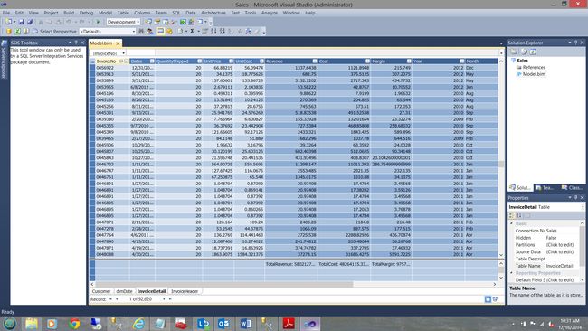
The project consist of four relational tables:
该项目包含四个关系表:
- Customer (containing customer details) 客户(包含客户详细信息)
- dimDate (a Date entity with week number, month number, etc.) dimDate(具有星期编号,月份编号等的Date实体)
- Invoice Header (the mommy a header has many details) 发票抬头(妈妈抬头有很多详细信息)
- Invoice Detail (the children) 发票明细(儿童)
This project model once deployed created the Analysis Services database with which we are now going to work.
部署后,该项目模型创建了Analysis Services数据库,我们现在将使用该数据库。
Let us begin by bringing up SQL Server Management Studio and log into a Tabular Instance that I have created.
让我们首先启动SQL Server Management Studio并登录到我创建的表格实例。
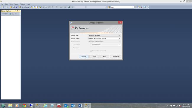
As a starting point we are going to have a quick look at how simple DAX queries are structured.
首先,我们将快速了解如何构造简单的DAX查询。
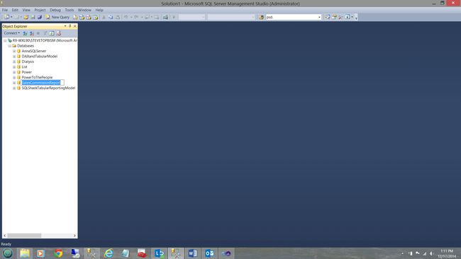
Having opened Analysis Services we note that there is a Tabular Analysis Services database called “SalesCommissionReport”. We shall be working with this database.
打开Analysis Services后,我们注意到有一个名为“ SalesCommissionReport”的表格分析服务数据库。 我们将使用此数据库。
We now open a ‘New Query’ (see above).
现在,我们打开一个“新查询”(见上文)。
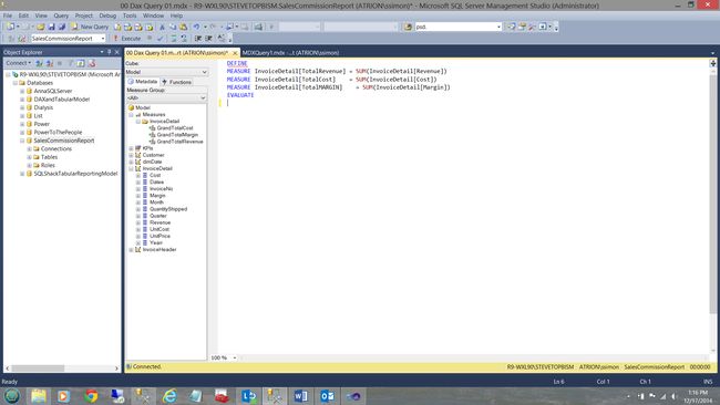
Note that the appearance of the query window is somewhat reminiscent of query work surface for multidimensional queries.
请注意,查询窗口的外观在某种程度上让人联想到多维查询的查询工作表面。
For our first example let us take a look at a simple business query.
对于第一个示例,让我们看一个简单的业务查询。
SQLShack Industries wishes to ascertain the total revenue, total cost and total margin for the varied invoiced items for a given time period.
SQLShack Industries希望确定给定时间段内各种发票项目的总收入,总成本和总利润。
In T-SQL we could express this in the following manner:
在T-SQL中,我们可以用以下方式表达这一点:
Select InvoiceNo, Datee as [Date], sum(Revenue) as Revenue, sum(Cost) as Cost,
Sum(Margin) as Margin from DaxAndTheTabularModel
Group by InvoiceNo, Datee
Now!! Let us now see (in easy steps) how we may construct this same query within the world of DAX.
现在!! 现在,让我们看看(简单的步骤)如何在DAX的世界中构造相同的查询。
To begin, we wish to create a piece of code that will sum the revenue, cost and margin. Let us see how this is done!
首先,我们希望创建一段将收入,成本和利润相加的代码。 让我们看看如何完成!

We note the command DEFINE at the start of the query. The astute reader will note that the ‘InvoiceDetail’ entity (see above) contains the fields “Revenue”, ”Cost” and “Margin”. These are the fields that we shall be using. Note that the three measures are created below the word DEFINE (see above (in the screen dump) and below for a snippet of the code).
我们在查询开始时注意到命令DEFINE 。 精明的读者会注意到,“ InvoiceDetail”实体(请参见上文)包含“收入”,“成本”和“保证金”字段。 这些是我们将要使用的字段。 请注意,这三个度量是在单词DEFINE下方创建的(请参见上方(在屏幕转储中)和下方的代码段)。
DEFINE
MEASURE InvoiceDetail[TotalRevenue] = SUM(InvoiceDetail[Revenue])
MEASURE InvoiceDetail[TotalCost] = SUM(InvoiceDetail[Cost])
MEASURE InvoiceDetail[TotalMARGIN] = SUM(InvoiceDetail[Margin])
A note is required at this point: The syntax for pulling fields from tabular databases is:
Entity[Attribute] as may be seen above. In our case “InvoiceDetail” is the entity and [TotalRevenue] the attribute.
此时需要注意:从表格数据库中提取字段的语法是:
实体[属性]如上所示。 在我们的例子中,“ InvoiceDetail”是实体,[TotalRevenue]是属性。
Now that we have created our ‘DEFINED’ fields it is time to construct the main query.
现在,我们已经创建了“ DEFINED”字段,是时候构造主查询了。
We first add the word ‘EVALUATE’ below our declaration of the MEASURES. EVALUATE corresponds to the word SELECT in traditional SQL code.
我们首先在措施声明的下方添加“评估”一词。 EVALUATE对应于传统SQL代码中的SELECT字。
Having issued the “EVALUATE” we now call for the fields that we wish to show within our query
发布“ EVALUATE”后,我们现在调用我们希望在查询中显示的字段
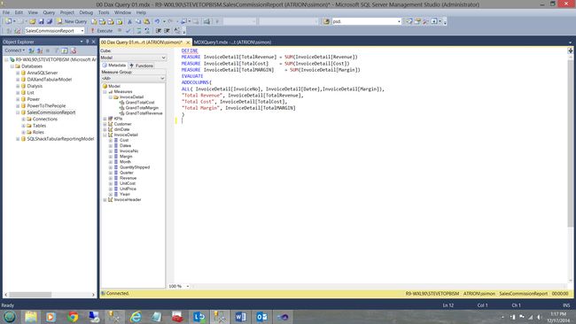
Note that we utilize the ADDCOLUMNS function to achieve this. The columns within the query may be seen above and a snippet of code may be seen below:
请注意,我们利用ADDCOLUMNS函数来实现这一点。 查询中的列可以在上方看到,代码片段可以在下方看到:
ADDCOLUMNS(
ALL( InvoiceDetail[InvoiceNo], InvoiceDetail[Datee],InvoiceDetail[Margin]),
"Total Revenue", InvoiceDetail[TotalRevenue],
"Total Cost", InvoiceDetail[TotalCost],
"Total Margin", InvoiceDetail[TotalMARGIN]
)
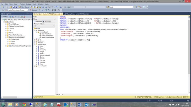
To complete the code and knowing that I want the data ordered by the invoice number, I add an ORDER BY statement.
为了完成代码并知道我想要按发票编号对数据进行排序,我添加了ORDER BY语句。
ORDER BY InvoiceDetail[InvoiceNo]
Thus our query is complete. Let us give it a spin!!
这样我们的查询就完成了。 让我们旋转一下!!
The results of the query may be seen below.
查询结果如下所示。
To recap
回顾
- DEFINE 定义
- Create your define fields 创建您的定义字段
- ADDCOLUMNS to your query including the defined fields 向您的查询添加列(包括定义的字段)
- Order by statement. 按语句排序。
We shall see how to use this for constructive usage in a few minutes.
我们将在几分钟内看到如何将此用于建设性使用。
另一个例子: (Another Example:)
In the next example I want to show you how easily one may obtain data from two or more entities (tables).
在下一个示例中,我想向您展示如何轻松地从两个或多个实体(表)获取数据。
After all in the real world, reporting queries normally do join to two or more tables. In our case we wish to look at ONLY data from the year 2010.
毕竟,在现实世界中,报表查询通常会联接到两个或多个表。 在我们的案例中,我们只希望查看2010年的数据。
Once again we start with the necessary EVALUATE command. We remember from above that this is the equivalent to the SELECT statement.
我们再次从必要的EVALUATE命令开始。 我们从上面记住,这等效于SELECT语句。
This time however we are going to utilize the “CALCULATETABLE” function. “CALCULATETABLE” evaluates a table expression in a context modified by the given filters (see below in yellow)
但是这次我们将利用“ CALCULATETABLE”功能。 “ CALCULATETABLE” 在由给定过滤器修改的上下文中评估表表达式(请参见下面的黄色)
|
EVALUATE CALCULATETABLE( SUMMARIZE(
‘InvoiceDetail’
,
‘dimDate’[datee]
,
‘Customer’[CustomerName]
, "Sales"
,
SUM( Invoicedetail[Revenue] ) )
,
InvoiceDetail[Yearr] = 2010 )
order
by
‘Customer’[CustomerName]
,
‘dimDate’[datee]
|
|
评估CALCULATETABLE(SUMMARIZE( 'InvoiceDetail' , 'dimDate' [datee] , 'Customer' [CustomerName] , “ Sales” , SUM (Invoicedetail [Revenue])) , InvoiceDetail [Yearr = 2010 ) 按 'Customer' [CustomerName ] 排序 ] , 'dimDate' [datee]
|
The astute reader will note that I am pulling the date from the ‘InvoiceDetail’ table (after all, an item is sold on a given date, not so? The customer name from the “Customer” table and the field “Sales” is sourced from the “InvoiceDetail” table.
精明的读者会注意到,我是从“ InvoiceDetail”表中提取日期的(毕竟,某个商品是在给定的日期出售的,不是吗?从“ Customer”表和“ Sales”字段中获取客户名称)从“ InvoiceDetail”表中。
When we run our query we find the following:
当我们运行查询时,我们发现以下内容:
Normally SQLShack Industries work solely with an invoice date only as opposed to the date and time. Often the time is meaningless as it is 00:00:00 etc. Invoice date and dollar values with thousandths and millionth of cents is also nonsense UNLESS one is in the banking industry. This said we shall “normalize” these values when we come to the report section of this article.
通常,SQLShack Industries仅使用发票日期而不是日期和时间来工作。 时间通常是没有意义的,因为它是00:00:00等。发票日期和千分之一与百万分之一的美元值也是胡说八道,除非是在银行业中。 这表示当我们进入本文的报告部分时,我们将“标准化”这些值。
我最喜欢的查询之一 (One of my FAVORITE queries)
One of the most beautiful features of using DAX is the ability to ascertain values for “the same period last year”.
使用DAX的最漂亮的功能之一就是能够确定“去年同期”的值。
In this query we are going to once again SUMMARIZE ( sum() ) the values and add the columns. This one however is a tad tricky to understand thus I am going to put the query together in pieces.
在此查询中,我们将再次对值进行SUMMARIZE(sum())并添加列。 但是,这一点很难理解,因此我将把查询分段。
Firstly, here are my DEFINE fields
首先,这是我的DEFINE字段
DEFINE
MEASURE 'Invoicedetail'[CalendarYear] =sumx('dimDate',Year('dimDate'[datee]) )
MEASURE 'InvoiceDetail'[PY Sales] =
CALCULATE( sumx('InvoiceDetail','Invoicedetail'[Revenue]),
 SAMEPERIODLASTYEAR( 'dimDate'[Datee] ))
The first line of code will give us the calendar year in which the items were sold. This helps the folks at SQLShack Industries set their frame of reference.
代码的第一行将为我们提供商品销售的日历年。 这有助于SQLShack Industries的人们设置参考框架。
The next line of code is a bit convoluted however simply put “PY Sales” is defined as ‘InvoiceDetail’[Revenue] FOR THE SAME DATE AND MONTH LAST YEAR! This is where the function
下一行代码有些复杂,但是简单地把“ PY Sales”定义为“ InvoiceDetail” [收入],用于去年的同一日期和月份! 这是功能
SAMEPERIODLASTYEAR( 'dimDate'[Datee] )
comes into play.
发挥作用。
Let us finally proceed to add our query columns so that we can view the result set of the query.
最后,让我们继续添加查询列,以便我们可以查看查询的结果集。
EVALUATE
ADDCOLUMNS(
FILTER(
SUMMARIZE(
'dimDate',
'dimDate'[datee],
'dimDate'[Month],
'dimDate'[Quarter],
'dimDate'[Weeknumber]
,"Sales: Today", sumx('InvoiceDetail','Invoicedetail'[Revenue]),
"Calender Year" ,'Invoicedetail'[CalendarYear]
),
//Filter the data
sumx('InvoiceDetail','Invoicedetail'[Revenue]) <> 0
),
// Add the past period DEFINED column
"Sales: Year ago Today", [PY Sales]
)
ORDER BY 'dimDate'[Datee], 'dimDate'[Month]
Once again, let us look at what each line of code achieves.
再次让我们看一下每一行代码可以实现什么。
Under “SUMMARIZE”, from the dimDate entity (table), pull the date, month, quarter and week number of the invoice date.
从dimDate实体(表)的“ SUMMARIZE”下,拉出发票日期的日期,月份,季度和星期数。
THEN
然后
"Sales: Today", sumx('InvoiceDetail','Invoicedetail'[Revenue]),
Sum the revenue for the date ( i.e. sum(revenue) group by date) for the CURRENT year under consideration.
所考虑的当前年度的日期的收入总和(即,按日期分组的总和(收入))。
We must remember that where current invoice year is 2012 then we create our “Last Year’s field” from the same date but for the year 2011. The important point being that aside from the lowest year’s data, EACH invoice date ‘has a turn’ to be a current date and the ‘same day and month’ BUT one year earlier (see the table below).
我们必须记住,当前发票年份是2012年,然后我们从同一日期创建2011年的“去年字段”。重要的一点是,除了年份最低的数据之外,每个发票日期都“轮到”了设置为当前日期,但设置为一年前的“同一天和月份”(但请参见下表)。
| Prior Year | Current Year |
| 20100101 | 20110101 |
| 20090101 | 20100101 |
| NULL | 20090101 |
| 去年 | 今年 |
| 20100101 | 20110101 |
| 20090101 | 20100101 |
| 空值 | 20090101 |
We also add the calendar year under consideration so that we know where we are in our table.
我们还会添加考虑中的日历年,以便我们知道我们在表中的位置。
As a means of showing how to create a query predicate, I am including a filter within this code. It probably does NOT make any business sense and is meant purely to be demonstrative.
为了说明如何创建查询谓词,我在此代码中包括了一个过滤器。 它可能没有任何商业意义,并且纯粹是出于说明目的。
//Filter the data
sumx('InvoiceDetail','Invoicedetail'[Revenue]) <> 0
Finally, I add the revenue from the prior period. NOTE that this is OUTSIDE of the SUMMARIZE function and the reason for this, is to avoid applying the conditions set within the SUMMARIZE function to the prior year’s figures.
最后,我加上上一时期的收入。 请注意,这不在SUMMARIZE函数之内,其原因是为了避免将SUMMARIZE函数中设置的条件应用于上一年的数字。
"Sales: Year ago Today", [PY Sales]
Finally we order our result set(by year, by month)
最后,我们对结果集进行排序(按年,按月)
ORDER BY 'dimDate'[Datee], 'dimDate'[Month]
Having now created three queries and knowing that we could have created a plethora more, at this point in time we should now have a look at how these queries may be utilized in a practical reporting scenario.
现在已经创建了三个查询,并且知道我们可以创建更多的查询,这时我们现在应该看看在实际的报告场景中如何利用这些查询。
使用DAX查询创建报告 (Creating reports with DAX queries)
We start (as we have in past discussions) by opening SQL Server Data Tools and by creating a new Reporting Services project. Should you be a bit uncertain how to create a Reporting Services project, please have a glance at one of my earlier articles where I do describe the project creation in detail OR contact me directly for some super “crib” notes!
首先,我们将打开SQL Server数据工具并创建一个新的Reporting Services项目(就像在过去的讨论中一样)。 如果您不确定如何创建Reporting Services项目,请浏览我的前一篇文章,其中确实详细描述了该项目的创建,或者直接与我联系以获得一些超级“婴儿”笔记!

We click OK to create the project. Once within the project, we right click on the “Report” folder and select “Add” and then “New Item” (see below).
我们单击确定以创建项目。 进入项目后,我们右键单击“ Report”文件夹,然后选择“ Add”,然后选择“ New Item”(见下文)。
The new item report screen is then brought into view (see below).
然后进入新项目报告屏幕(见下文)。
I select “Report” , give my report a name and the click “Add”.
我选择“报告”,给我的报告起一个名字,然后单击“添加”。

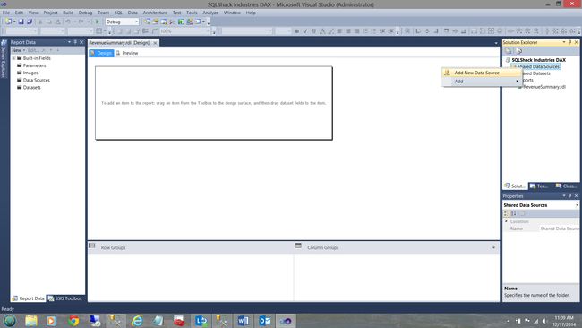
We now find ourselves back at the report “drawing surface”.
现在,我们回到报告“图纸”上。
Our first task is to create a “Shared Data Source” (as we have in past articles).
我们的第一个任务是创建一个“共享数据源”(就像过去的文章一样)。
I right click on the “Shared Data Source” folder and select “Add New Data Source”
我右键单击“共享数据源”文件夹,然后选择“添加新数据源”
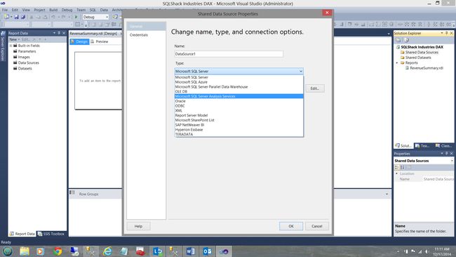
The “Shared Data Source” properties box is shown (see below).
显示“共享数据源”属性框(请参见下文)。
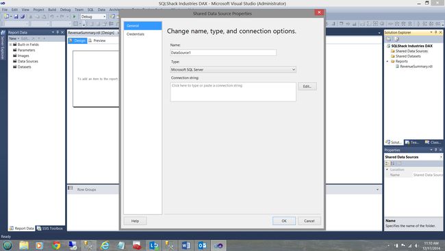
We CHANGE the “Type” box to “Microsoft SQL Server Analysis Services” (see below).
我们将“类型”框更改为“ Microsoft SQL Server Analysis Services”(请参见下文)。
We now click the “Edit” button and the “Change name, type and connection options” dialog box is displayed (see below).
现在,我们单击“编辑”按钮,并显示“更改名称,类型和连接选项”对话框(如下所示)。
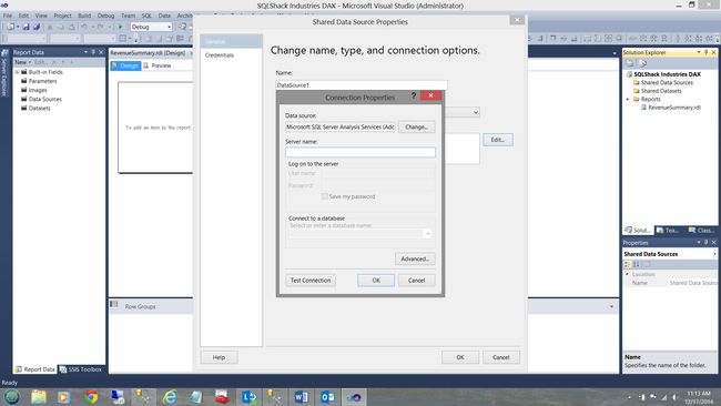
I now set my server and choose our “SalesCommissionReport” database and test the connection (see below).
现在,我设置服务器并选择“ SalesCommissionReport”数据库并测试连接(请参见下文)。
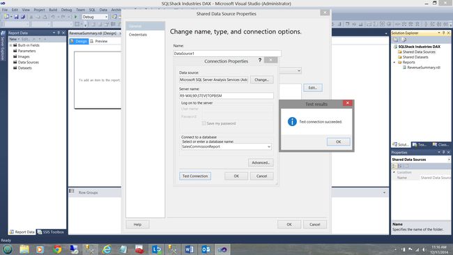
We click OK, OK and OK to exit and we are now ready to go!!
我们单击“确定”,“确定”和“确定”退出,我们现在可以开始了!
Once back on the drawing surface our first task is to create a data set to hold data PULLED from the Analysis Services tabular database. As I have described in earlier articles, a dataset may be likened to a bucket that is filled with water via a hose pipe coming from the faucet on the outside wall of your house. We then use the bucket of water to water the plants and in our case (with data) to populate our report(s).
回到图纸表面后,我们的首要任务是创建一个数据集,以保存来自Analysis Services表格数据库的PULLED数据。 正如我在之前的文章中所描述的,数据集可以比喻成一个桶,该桶通过来自房屋外墙水龙头的软管通过水管充满水。 然后,我们使用一桶水为植物浇水,在这种情况下(包含数据)填充报告。
AT THIS POINT I WOULD ASK THAT WE FOLLOW THE NEXT STEPS CAREFULLY as Microsoft has still to properly define a proper method to create TABULAR DATA sets. We MUST utilize a work-around.
在这一点上,我会建议我们遵循以下步骤,因为Microsoft仍必须正确定义创建TABULAR数据集的适当方法 。 我们必须利用一种变通方法。
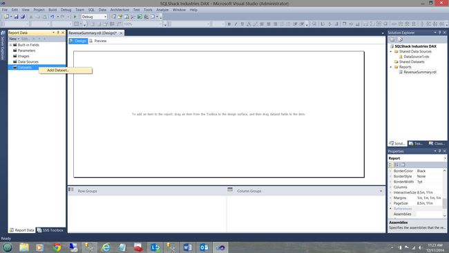
We right click on the “Data Set” folder and select “Add Dataset”
我们右键单击“数据集”文件夹,然后选择“添加数据集”
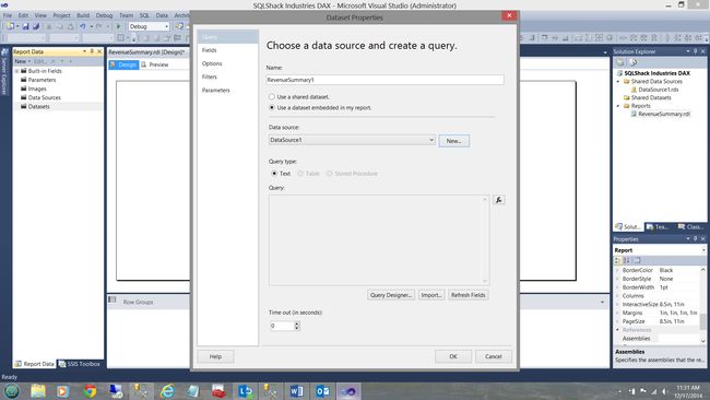
The “Choose a data source and create a query” dialog box appears (see below).
出现“选择数据源并创建查询”对话框(见下文)。
I give my dataset a name (see above) and click “New” to create a new local data source (for this report only) see above.
我给数据集命名(请参见上文),然后单击“新建”以创建新的本地数据源(仅针对此报告),请参见上文。
The “New data source” box is brought up and I select our share data source that we defined a few seconds ago (see below).
出现“新数据源”框,然后选择几秒钟前定义的共享数据源(见下文)。

I click OK to exit the “Data Source” dialog. We find ourselves back at the “Data Set” dialog box.
我单击“确定”退出“数据源”对话框。 我们回到“数据集”对话框。
Now our queries are in fact text and the eagle-eyed reader will note that the “Query” dialog box is “greyed out”. Let the fun and games begin!!!
现在我们的查询实际上是文本,老鹰眼的读者会注意到“查询”对话框是“灰色”。 让乐趣和游戏开始!!!
What is required to get Reporting Services to accept our DAX code is to select the “Query Designer” button (see above).
要使Reporting Services接受我们的DAX代码,需要选择“查询设计器”按钮(请参见上文)。
Clicking the “Query Designer” button brings up the “Query Designer” dialog box.
单击“查询设计器”按钮将弹出“查询设计器”对话框。
At this point we MUST SELECT “COMMAND TYPE DMX”. The button is found immediately above the “Command Type DMX” tool tip (see below).
此时,我们必须选择“命令类型DMX”。 该按钮位于“ Command Type DMX”工具提示的上方(请参见下文)。
We are then informed that “Switching from MDX to DMX will result in losing all current design content. Do you want to proceed?” We click “Yes”.
然后我们得知:“从MDX切换到DMX将导致丢失所有当前的设计内容。 您要继续吗?” 我们点击“是”。
We now choose to go into design mode (see below). The button is found immediately above the “Design Mode” tool tip (see below).
现在,我们选择进入设计模式(见下文)。 该按钮位于“设计模式”工具提示的上方(请参见下文)。
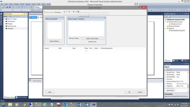
We are now finally able to insert our query (see below).
现在,我们终于可以插入查询了(见下文)。

Click OK to complete the process.
单击确定以完成该过程。
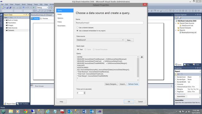
We are returned to our create data set screen. We now click “Refresh Fields” in the lower right hand portion of the screen dump above. We now select the “Fields” tab in the upper left have portion of the screen dump below.
我们返回到创建数据集屏幕。 现在,我们在上方屏幕转储的右下角单击“刷新字段”。 现在,我们选择左上方屏幕顶部的“字段”选项卡。

The fields for our query may be seen above. Click OK to leave the “Data Set” dialog.
我们查询的字段可以在上方看到。 单击确定退出“数据集”对话框。
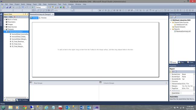
We find ourselves back on the drawing surface with our data set created.
我们发现自己有了创建的数据集,回到了图纸表面。
Next, we drag a “Matrix” onto the drawing surface (see below).
接下来,我们将“矩阵”拖到绘图表面上(见下文)。
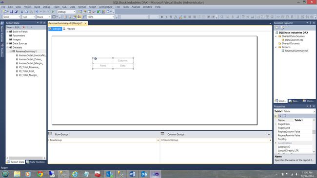
We now remove the “Column Groups” by right clicking on the [Column Group] and select removing grouping only (see below).
现在,我们通过右键单击[Column Group]并选择“仅删除分组”来删除“ Column Groups”(请参见下文)。
We click OK to accept and leave the “Delete Group” dialog.
我们单击“确定”接受并离开“删除组”对话框。

We now insert four more columns by right clicking on the top margin of the matrix (shown in black above).
现在,我们通过右键单击矩阵的上边距再插入四列(如上黑色所示)。

Our finished surface may be seen above.
我们完成的表面可以在上面看到。
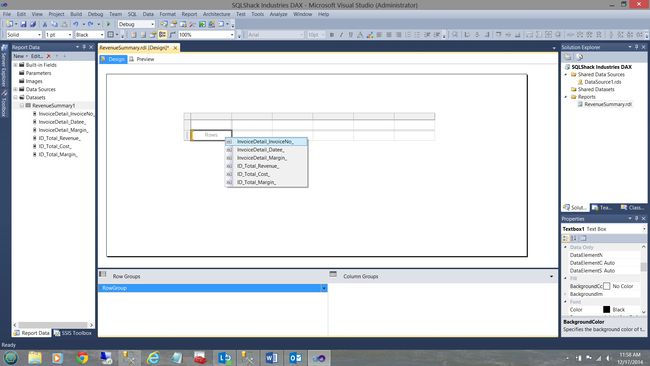
We now insert our first field (see above).
现在,我们插入第一个字段(请参见上文)。
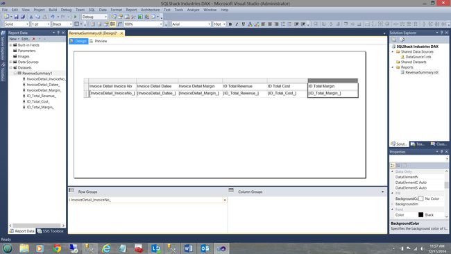
The screen shot above shows the matrix once all of the fields have been populated.
一旦填充了所有字段,上面的屏幕快照就会显示矩阵。
Looking at the column headings, we find them a bit cryptic. We shall change them as follows (see below).
查看列标题,我们发现它们有点神秘。 我们将对其进行如下更改(请参见下文)。

Finally, we wish to change the ‘Hum Drum’ appearance by adding some fill to our text boxes. We choose “Khaki” for the headers and “Light Grey” for the values themselves.
最后,我们希望通过在文本框中添加一些填充来更改“嗡嗡声鼓”的外观。 我们为标题选择“卡其色”,为值本身选择“浅灰色”。
..and
..和
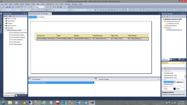
The “value” or result text boxes are filled in with Light Grey.
“值”或结果文本框用浅灰色填充。
Let us give our report a whirl by selecting “Preview”
让我们通过选择“预览”来给我们的报告一个旋转
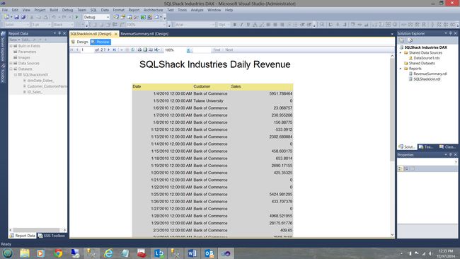
Here are the results. A mentioned earlier, we must now convert the date times to dates and have the dollar fields show only two decimal places.
这是结果。 前面提到过,我们现在必须将日期时间转换为日期,并且美元字段仅显示两位小数。
We do so as follows:
我们这样做如下:
Right clicking on the “datee” field “result box”, bring up the Textbox Properties dialog box (see below).
右键单击“日期”字段的“结果框”,弹出“文本框属性”对话框(如下所示)。
We select “Number”,”Date” and choose a format and click OK to finish. Our report now looks as follows.
我们选择“数字”,“日期”,然后选择一种格式,然后单击“确定”完成。 现在,我们的报告如下。

Changing the “dollar” values, we now see the following:
更改“美元”值后,我们现在看到以下内容:
And the final report…
最后的报告
Thus our report is complete and ready for the production environment!!!
因此,我们的报告是完整的,可用于生产环境!!!
创建第二和第三报告 (Creating reports number two and three)
I have taken the liberty of creating these two reports with the remaining two queries that we created above. The report creating process is the same as we have just seen for our Revenue Summary report.
我已经自由创建了两个报表,并使用了上面创建的其余两个查询。 报告创建过程与我们在“收入摘要”报告中看到的过程相同。
And last but not least our “Same Period Last Year” report.
最后但并非最不重要的是我们的“去年同期”报告。
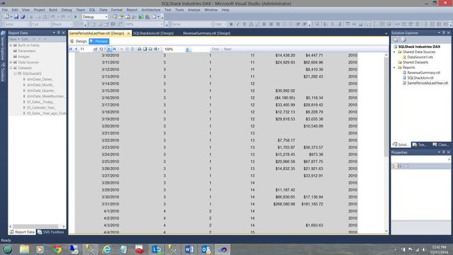
Thus we have completed our first venture into utilizing DAX expressions for queries which will be eventually utilized for reporting. Further they may be utilized with any data extracts utilizing Excel. But that is for another day.
因此,我们完成了将DAX表达式用于查询的最终尝试,并将最终用于报告。 此外,它们可以与任何使用Excel的数据提取一起使用。 但这是另一天。
结论 (Conclusions)
With Power BI being the “Top of the pops” for reporting purposes within major industries and enterprises, it is and will become necessary for most SQL developers and BI specialists alike to become more fluent with the DAX language. More so for those enterprises that are heavily dependent on reporting via Excel.
由于Power BI成为主要行业和企业中用于报告目的的“流行之首”,因此对于大多数SQL开发人员和BI专家而言,变得越来越熟练使用DAX语言是有必要的,并且将有必要。 对于那些严重依赖于通过Excel进行报告的企业而言,尤其如此。
Whilst DAX seems complex at first, it is fairly easy to learn and in doing so, you will put yourself ahead of the curve.
虽然DAX乍一看似乎很复杂,但它很容易学习,这样做的话,您将处于领先地位。
Happy programming!!!
编程愉快!!!
翻译自: https://www.sqlshack.com/getting-started-with-data-analysis-expressions-sql-server/