监督学习-分类模型1-线性分类器(Linear Classifiers)
打算把《python机器学习-通往kaggle竞赛之路》手动敲一遍,
- 加强机器学习各个算法和操作步骤的代码记忆
- 熟悉使用markdown的公式语法,便捷工具mathpix
- 熟悉机器学习专有名称和英文表达
- 将python2代码转为python3代码
- 修改过期的模块引用,如from sklearn.cross_validation改为 from sklearn.model_selection
造导弹,自主研发需要4年,模仿只需1年 - 《钱学森》
模型介绍:线性分类器(linear classification),是一种假设特征与分类结果存在线性关系的模型。这个模型通过累加计算每个维度的特征与各自权重的乘机来帮助类别决策。
如果我们定义 $ x =
f ( w , x , b ) = w T x + b ( 1 ) f(w,x,b)=w^Tx+b (1) f(w,x,b)=wTx+b(1)
这里的 f ∈ R f \in R f∈R ,取值范围分布在整个实数域中。然而,我们要处理的最简单的二分类问题希望$ f \in { 0,1}$,因此需要一个函数把原先的 f ∈ R f \in R f∈R 映射到(0,1)。于是用到了逻辑斯蒂(logistic)函数:
g ( z ) = 1 1 + e − z ( 2 ) g(z)=\frac{1}{1+e^{-z}} (2) g(z)=1+e−z1(2)
这里的 z ∈ R z \in R z∈R并且 g ∈ ( 0 , 1 ) g \in (0,1) g∈(0,1),并且其函数图像如图2-2所示。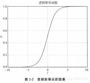
综上,如果将 z z z替换为 f f f,整合方程式(1)和方程式(2),就获得了一个经典的线性分类器,逻辑斯蒂回归模型(Logistic Regression):
h w , b ( x ) = g ( f ( w , x , b ) ) = 1 1 + e − f = 1 1 + e − ( w T x + b ) ( 3 ) h_{w,b}(x)=g(f(w,x,b))=\frac{1}{1+e^{-f}}=\frac{1}{1+e^{-(w^Tx+b)}} (3) hw,b(x)=g(f(w,x,b))=1+e−f1=1+e−(wTx+b)1(3)
从图2-2中便可以观察到该模型如何处理一个待分类的特征向量:如果 z = 0 z=0 z=0,那么 g = 0.5 g=0.5 g=0.5;若 z < 0 z<0 z<0则 g < 0.5 g<0.5 g<0.5,这个特征向量被判别为一类;反之,若 z > 0 z>0 z>0则 g > 0.5 g>0.5 g>0.5,其被归为另外一类。
当使用一组 m m m个用于训练的特征向量 X = < x 1 , x 2 , ⋅ ⋅ ⋅ , x m > X=<x^1,x^2,···,x^m> X=<x1,x2,⋅⋅⋅,xm>和其所对应的分类目标 y = < y 1 , y 2 , ⋅ ⋅ ⋅ , y m > y=<y^1,y^2,···,y^m> y=<y1,y2,⋅⋅⋅,ym>,我们希望逻辑斯蒂模型可以在这组训练集上取得最大似然估计(Maximum Likelihood)的概率 L ( w , b ) L(w,b) L(w,b)。或者说,至少要在训练集上表现如此:
argmax x , b L ( w , b ) = argmax x , b ∏ i = 1 m ( h x , b ( i ) ) y ′ ( 1 − h x , b ( i ) ) 1 − y i \underset{x, b}{\operatorname{argmax}} L(w, b)=\underset{x, b}{\operatorname{argmax}} \prod_{i=1}^{m}\left(h_{x, b}(i)\right)^{y^{\prime}}\left(1-h_{x, b}(i)\right)^{1-y^{i}} x,bargmaxL(w,b)=x,bargmaxi=1∏m(hx,b(i))y′(1−hx,b(i))1−yi
为了学习到决定模型的参数(Parameters),即系数 w w w和截距 b b b,我们采用随机梯度上升算法(stochastic gradient ascend)。
性能测评
二分类任务下,预测结果(Predicted Condition)和正确标记(True Condition)之间存在4种不同的组合,构成混淆矩阵(Confusion Matrix),如图2-4所示。
- 恶性肿瘤为阳性 Positive
- 良性肿瘤为阴性 Negative
- 预测正确的恶行肿瘤为真阳性 True Positive
- 预测正确的良性肿瘤为真阴性 True Negative
- 良性肿瘤误判为恶行肿瘤为假阳性 False Positive
- 恶性肿瘤漏报成良性肿瘤为假阴性 False Nagative
- 准确性 Accuracy
A c c u r a c y = T P + T N T P + T N + F P + F N ( 5 ) Accuracy=\frac{TP+TN}{TP+TN+FP+FN} (5) Accuracy=TP+TN+FP+FNTP+TN(5) - 精确率 Precision
P r e c i s i o n = T P T P + F P ( 6 ) Precision=\frac{TP}{TP+FP} (6) Precision=TP+FPTP(6) - 召回率 Recall
R e c a l l = T P T P + F N ( 7 ) Recall= \frac{TP}{TP+FN}(7) Recall=TP+FNTP(7) - F1指标,召回率与精确率的调和平均数 F1 measure
F 1 m e a s u r e = 2 1 P r e c i s i o n + 1 R e c a l l ( 8 ) F1 \ measure=\frac{2}{\frac{1}{Precision}+\frac{1}{Recall}}(8) F1 measure=Precision1+Recall12(8)

编程实践
良/恶行乳腺癌肿瘤预测
数据地址:https://archive.ics.uci.edu/ml/machine-learning-databases/breast-cancer-wisconsin/
# 导入pandas与numpy工具包。
import pandas as pd
import numpy as np

# 创建特征列表。
column_names = ['Sample code number', 'Clump Thickness', 'Uniformity of Cell Size', 'Uniformity of Cell Shape', 'Marginal Adhesion', 'Single Epithelial Cell Size', 'Bare Nuclei', 'Bland Chromatin', 'Normal Nucleoli', 'Mitoses', 'Class']

# 使用pandas.read_csv函数从互联网读取指定数据。
data = pd.read_csv('https://archive.ics.uci.edu/ml/machine-learning-databases/breast-cancer-wisconsin/breast-cancer-wisconsin.data', names = column_names )

# 将?替换为标准缺失值表示。
data = data.replace(to_replace='?', value=np.nan)
# 丢弃带有缺失值的数据(只要有一个维度有缺失)。
data = data.dropna(how='any')
# 输出data的数据量和维度。
data.shape

# 使用sklearn.model_selection里的train_test_split模块用于分割数据。
from sklearn.model_selection import train_test_split
# 随机采样25%的数据用于测试,剩下的75%用于构建训练集合。
X_train, X_test, y_train, y_test = train_test_split(data[column_names[1:10]], data[column_names[10]], test_size=0.25, random_state=33)
# 查验训练样本的数量和类别分布。
y_train.value_counts()
# 查验测试样本的数量和类别分布。
y_test.value_counts()

# 从sklearn.preprocessing里导入StandardScaler。
from sklearn.preprocessing import StandardScaler
# 从sklearn.linear_model里导入LogisticRegression与SGDClassifier。
from sklearn.linear_model import LogisticRegression
from sklearn.linear_model import SGDClassifier

# 标准化数据,保证每个维度的特征数据方差为1,均值为0。使得预测结果不会被某些维度过大的特征值而主导。
ss = StandardScaler()
X_train = ss.fit_transform(X_train)
X_test = ss.transform(X_test)

# 初始化LogisticRegression与SGDClassifier。
lr = LogisticRegression()
sgdc = SGDClassifier()

# 调用LogisticRegression中的fit函数/模块用来训练模型参数。
lr.fit(X_train, y_train)
# 使用训练好的模型lr对X_test进行预测,结果储存在变量lr_y_predict中。
lr_y_predict = lr.predict(X_test)

# 调用SGDClassifier中的fit函数/模块用来训练模型参数。
sgdc.fit(X_train, y_train)
# 使用训练好的模型sgdc对X_test进行预测,结果储存在变量sgdc_y_predict中。
sgdc_y_predict = sgdc.predict(X_test)

# 从sklearn.metrics里导入classification_report模块。
from sklearn.metrics import classification_report

# 使用逻辑斯蒂回归模型自带的评分函数score获得模型在测试集上的准确性结果。
print('Accuracy of LR Classifier:', lr.score(X_test, y_test))
# 利用classification_report模块获得LogisticRegression其他三个指标的结果。
print(classification_report(y_test, lr_y_predict, target_names=['Benign', 'Malignant']))

 # 使用随机梯度下降模型自带的评分函数score获得模型在测试集上的准确性结果。
print('Accuarcy of SGD Classifier:', sgdc.score(X_test, y_test))
# 利用classification_report模块获得SGDClassifier其他三个指标的结果。
print(classification_report(y_test, sgdc_y_predict, target_names=['Benign', 'Malignant']))
特点分析
本次模型使用了LogisticRegression和SGDClassifier。前者对参数的计算采用精确解析的方式,计算时间长但是产出的模型性能略高;后者采用随机梯度上升算法估计模型参数,计算时间短但是产出的模型性能略低。一般而言,对于训练数据10万量级上的,考虑时间,推荐用随机梯度算法对模型参数进行估计。