吴恩达机器学习第二周编程作业（Python实现）

课程作业 提取码：3szr

1、单元线性回归
ex1.py

from matplotlib.colors import LogNorm
from mpl_toolkits.mplot3d import Axes3D
from computeCost import *
from plotData import *
print('Plotting Data...')
data=np.loadtxt('./data/ex1data1.txt',delimiter=',')#加载txt格式数据集 每一行以“，”分隔

X=data[:,0]
y=data[:,1]

m=y.size

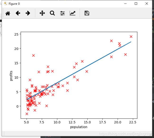
plt.figure(0)
plot_data(X,y)
# input()

print('Running Gradient Descent...')
X=np.c_[np.ones(m),X]
theta=np.zeros(2)

iterations=1500
alpha=0.01
print('Initial cost: '+str(compute_cost(X,y,theta))+'(This value should be about 32.07')
theta,J_history =gradient_descent(X,y,theta,alpha,iterations)
print('Theta found by gradient descent:'+str(theta.reshape(2)))

plt.figure(0)
line1, =plt.plot(X[:,1],np.dot(X,theta),label='Linear Regression')
plot_data(X[:,1],y)
plt.legend(handles=[line1])

input('Program paused. Press ENTER to continue')

predict1=np.dot(np.array([1,3.5]),theta)
print('For population=35,000,we predict a profit of {:0.3f}(This value should be about 4519.77)'.format(predict1*10000))
predict2=np.dot(np.array([1,7]),theta)
print('For population = 70,000, we predict a profit of {:0.3f} (This value should be about 45342.45)'.format(predict2*10000))
input('Program paused. Press ENTER to continue')

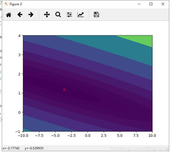
print('Visualizing J(theta_0,theta_1)...')
theta0_vals=np.linspace(-10,10,100)
theta1_vals=np.linspace(-1,4,100)
J_vals=np.zeros((theta0_vals.shape[0],theta1_vals.shape[0]))
print(theta0_vals.shape[0])
print(theta1_vals.shape[0])


for i in range(0,theta0_vals.shape[0]):
    for j in range(0,theta1_vals.shape[0]):
        t=np.array([theta0_vals[i],theta1_vals[j]])
        J_vals[i][j]=compute_cost(X,y,t)
J_vals=np.transpose(J_vals)
fig=plt.figure(1)
ax=Axes3D(fig)
xs,ys=np.meshgrid(theta0_vals,theta1_vals)
plt.title("Visualizing J(theta_0,theta_1)")

ax.plot_surface(xs,ys,J_vals)
ax.set_xlabel('$\theta_0$',color='r')
ax.set_ylabel('$\theta_1$',color='r')

plt.show()

plt.figure(2)
lvls=np.logspace(-2,3,20)
plt.contourf(xs,ys,J_vals,10,levels=lvls,normal=LogNorm())

plt.plot(theta[0], theta[1], c='r', marker="x")

plt.show()

plotData.py

import matplotlib.pyplot as plt
def plot_data(x,y):
    plt.scatter(x,y,marker='x',s=50,c='r',alpha=0.8)
    plt.xlabel('population')
    plt.ylabel('profits')
    plt.show()

computeCost.py(梯度下降函数包含在内）

import numpy as np
def h(X,theta):
    return X.dot(theta)
def compute_cost(X,y,theta):
    m=y.size
    prediction=h(X,theta)
    # cost=sum(np.power(prediction-y,2))/(2*m)
    cost = (prediction - y).dot(prediction - y) / (2 * m)
    return cost
def gradient_descent(X,y,theta,alpha,num_iters):
    m=y.size
    J_history=np.zeros(num_iters)
    for i in range(0,num_iters):
        # theta=theta-(alpha/m)*sum((h(X,theta)-y).dot(X))
        theta=theta-(alpha/m)*(h(X,theta)-y).dot(X)
        J_history[i]=compute_cost(X,y,theta)

    return theta,J_history