keras LSTM网络的实例和解释
LSTM网络的实例和解释
注: 本文主要参考 LSTM实例中sin函数和股票的预测,本文对该文章进行了进一步的解释,以及该文章所提供的源码中bug的纠正和完善。
除了本篇论文中涉及的实例,更多可以学习的LSTM实例见人数预测和人类行为预测。
keras LSTM函数使用实例和注释
官方文档给出的LSTM函数的使用规则参考价值不大,因为参量过于复杂,而且解释很少,参考几个开源代码,总结出如下的几种使用方法,不足之处请道友不吝赐教!
- 用法1: LSTM(output_dim=CELL_SIZE, input_dim=INPUT_SIZE, input_length=TIME_STEPS, return_sequences=Flase,stateful=FALSE)
output_dim:输出单个样本的特征值的维度
input_dim: 输入单个样本特征值的维度
input_length: 输入的时间点长度
return_sequences:布尔值,默认False,控制返回类型。若为True则返回整个序列,否则仅返回输出序列的最后一个输出,即当return_sequences取值为True时,网络输入和输出的时间长度TIME_STEPS保持不变,而当return_sequences取值为FALSE时,网络输出的数据时间长度为1。例如输入数据时间长度为5,输出为一个结果。
stateful: 布尔值,默认为False,若为True,则一个batch中下标为i的样本的最终状态将会用作下一个batch同样下标的样本的初始状态。当batch之间的时间是连续的时候,就需要stateful取True,这样batch之间时间连续。
实例程序如下:
model = Sequential()
model.add(LSTM(32, input_dim=64, input_length=10, return_sequences=True))
# note that you only need to specify the input size on the first layer.
# for subsequent layers, no need to specify the input size:
model.add(LSTM(16, return_sequences=True))
model.add(LSTM(10))
上面的程序构建的网络,输入数据的形状为10个时间长度,每一个时间点下的样本数据特征值维度是64。
第一层LSTM 输出的数据,时间维度仍然是10,每一个时间点下的样本数据特征值维度是32。
第二层LSTM 输出的数据,时间维度仍然是10,每一个时间点下的样本数据特征值维度是16。
第三层LSTM 输出的数据,由于return_sequences默认为FALSE,时间维度变成1,每一个时间点下的样本数据特征值维度是10。
- 用法2: LSTM(output_dim=CELL_SIZE, batch_input_shape=(BATCH_SIZE, TIME_STEPS, INPUT_SIZE) return_sequences=Flase)
用法2相比于用法1在输入数据中多指定了BATCH_SIZE的大小,但实际使用的时候不太方便,所以本人更倾向于用法1,然后BATCH_SIZE在训练的时候在函数model.fit中指定,如下:
model.fit(
    X_train,
    y_train,
    batch_size=512,
    nb_epoch=1,
    validation_split=0.05)
LSTM导入数据的结构与产生实例
本例参考源码,主要改动在于载入数据读取出来的是字符串,需要转换成float。
def load_data(filename, seq_len, normalise_window):
    f = open(filename, 'rb').read()
    data = f.decode().split('\n')

    #读取出来的是字符串,需要转换成float
    data_float = [float(da) for da in data]

    #此处长度+1,是因为需要留下最后的一个时间点作为训练的标签,即最后一个时间点被拆分出来作为y。
    #构造出来的result数组,每一行都比上一行平移了一个时间点
    sequence_length = seq_len + 1
    result = []
    for index in range(len(data_float) - sequence_length+1):
        result.append(data_float[index: index + sequence_length])
    #如果是股票,就需要归一化,具体的程序normalise_windows可以参考完整代码。
    if normalise_window:
        result = normalise_windows(result)

    result = np.array(result)
    #拆分出0.9作为测试集
    row = round(0.9 * result.shape[0])
    train = result[:int(row), :]
    #将训练集的数据打乱顺序
    #np.random.shuffle(train)

    #保留最后一个时间点为标签
    x_train = train[:, :-1]
    y_train = train[:, -1]

    x_test = result[int(row):, :-1]
    y_test = result[int(row):, -1]

    x_train = np.reshape(x_train, (x_train.shape[0], x_train.shape[1], 1))
    x_test = np.reshape(x_test, (x_test.shape[0], x_test.shape[1], 1))

return [x_train, y_train, x_test, y_test]- 预测方案1: 每一轮预测输入包含真实的50个时间点的数据,只预测后面的一个点
预测部分的代码如下:
def predict_point_by_point(model, data):
    #Predict each timestep given the last sequence of true data, in effect only predicting 1 step ahead each time
    predicted = model.predict(data)
    predicted = np.reshape(predicted, (predicted.size,))
    return predicted
sin函数预测的结果如下:

事实上,我们用同样的程序去预测股票,得到的结果是:

可以看到之预测紧接着的一个时间点的数据看上去预测效果非常的理想。但实际上,此处有陷阱。
参考原文
Running the data on a single point-by-point prediction as mentioned above gives something that matches the returns pretty closely. But this is deceptive! Why? Well if you look more closely, the prediction line is made up of singular prediction points that have had the whole prior true history window behind them. Because of that, the network doesn’t need to know much about the time series itself other than that each next point most likely won’t be too far from the last point. So even if it gets the prediction for the point wrong, the next prediction will then factor in the true history and disregard the incorrect prediction, yet again allowing for an error to be made.
其大意是,即便有时候只预测一个后面一个时间点的曲线看上去好像很有效果,但是实际上,由于每次的下一个时间点数据距离上一个时间点很近,所以网络就算没有学习出变化的规律,只有在上一个时间点附近随机产生 一个点,那么最后的结果距离真实的数据也不会相差很大,看上去就好像能预测出来规律一样,实际上可能网络只是在上一个时间点的附近随机产生了一个数据。
为了探索网络是否能真正的预测出数据的变化规律,我们可以采用预测值预测下一步的预测值,来探索网络是否能继续预测下去,即如下文方案2。
- 预测方案2: 每一轮输入数据是一个逐步滑动的窗口,初始输入是长度为50的时间序列,每一次预测后,将刚预测出来的数据加到时间序列末尾,并将序列首部的第一个时间数据移去,逐步滑动,无限期预测后面的数据
预测部分的代码如下:
def predict_sequence_full(model, data, window_size):
    #Shift the window by 1 new prediction each time, re-run predictions on new window
    curr_frame = data[0]
    predicted = []
    for i in range(len(data)):
        predicted.append(model.predict(curr_frame[newaxis,:,:])[0,0])
        curr_frame = curr_frame[1:]
        curr_frame = np.insert(curr_frame, [window_size-1], predicted[-1], axis=0)
    return predicted
sin函数预测的结果如下:
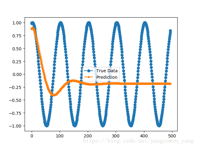
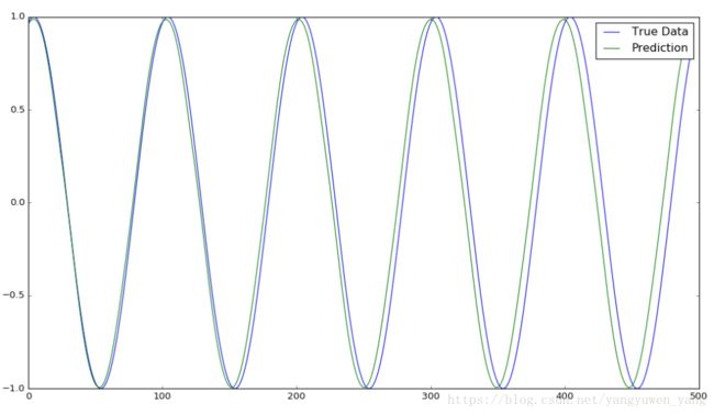
此处有一个我目前还是很疑惑的地方,事实上,根据作者提供的代码 中readme中的图示,表示sin函数长时间持续预测出来的结果应当是如下:
也就是说,网络应当是能够正确预测sin函数的长时间持续规律,但实际上,我使用作者提供的这一份代码,跑出来的却是上上一幅图的效果,也就是预测失败,基本后期到达sin曲线的中间线后保持稳定。我使用的代码就是作者提供的,但是却并没有得到作者的效果。为了方便读者试验,我将我的完整代码上传至这里,除了load_data部分函数有数据类型的纠正,其他部分代码均无改动。
股票的预测:
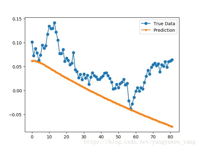
可以发现,上述的曲线都不具备长期预测的能力。
- 预测方案3:与方案2都是预测一次,滑动一次窗口,用预测值填充窗口。不同之处在于,滑动窗口到窗口中只有一个真实数据时,就需要重新输入一次真实数据组成的长度为50的序列窗口
预测部分的代码如下:
def predict_sequences_multiple(model, data, window_size, prediction_len):
    #Predict sequence of 50 steps before shifting prediction run forward by 50 steps
    prediction_seqs = []
    for i in range(int(len(data)/prediction_len)):
        curr_frame = data[i*prediction_len]
        predicted = []
        for j in range(prediction_len):
            predicted.append(model.predict(curr_frame[newaxis,:,:])[0,0])
            curr_frame = curr_frame[1:]
            curr_frame = np.insert(curr_frame, [window_size-1], predicted[-1], axis=0)
        prediction_seqs.append(predicted)
    return prediction_seqs
此处分析暂时保留,未待完续。