二手车价预测分析

数据分析：二手车价格预测分析

目录

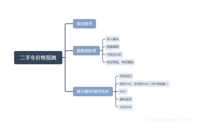
一、项目要求

1，背景
二手车报价在二手车交易中对消费者有着至关重要的意义，为了大致了解二手车评估价格，消费者直接利用网上评估也是比较常见的方法，可以避免被‘坑’。
汽车网站提供的在线评估系统可以为消费者了解市场、了解价格提供了重要的依据。

2，目标
借助二手车交易数据，建立准确的二手车价格预估回归模型，可以为网站在线评估系统汽车定价提供依据。

3，内容
根据二手车市场交易相关数据，分析不同特征与价格之间的关系，使用多类算法（线性回归、支持向量机、多层感知机、随机森林、XGBoost）创建回归模型，预测二手车交易价格。

二、数据预处理

导入模块

import pandas as pd
import numpy as np
import matplotlib.pyplot as plt
import seaborn as sns
from scipy.stats import norm    

from sklearn.preprocessing import StandardScaler
from sklearn.model_selection import train_test_split
from sklearn.model_selection import GridSearchCV
from sklearn.linear_model import LinearRegression
from sklearn.svm import LinearSVR
from sklearn.svm import SVR
from sklearn.neural_network import MLPRegressor
from sklearn.ensemble import RandomForestRegressor
from xgboost import XGBRegressor
from sklearn.metrics import r2_score
from sklearn.model_selection import cross_val_score


#可视化的中文处理
plt.rcParams['font.sans-serif'] = 'Microsoft YaHei'
plt.rcParams['axes.unicode_minus'] = False
plt.style.use('ggplot')

导入数据

#导入数据
car=pd.read_csv(r'second_cars_info.csv',encoding='gbk') 
#数据无缺失值。
car.info() 
<class 'pandas.core.frame.DataFrame'>
RangeIndex: 11281 entries, 0 to 11280
Data columns (total 7 columns):
Brand            11281 non-null object
Name             11281 non-null object
Boarding_time    11281 non-null object
Km               11281 non-null object
Discharge        11281 non-null object
Sec_price        11281 non-null float64
New_price        11281 non-null object
dtypes: float64(1), object(6)

#查看数据大致信息内容，变量包括汽车品牌Brand、汽车款式Name、上牌时间Boarding_time、行驶里程数Km、排放标准Discharge、二手价格Sec_price和新车价格New_price，其中只有二手价格Sec_price是数值变量。
car.head()
  Brand                            Name 		Boarding_time        Km 	Discharge  
0    奥迪         奥迪A6L 2006款 2.4 CVT 舒适型       2006年8月   9.00万公里        国3   
1    奥迪         奥迪A6L 2007款 2.4 CVT 舒适型       2007年1月   8.00万公里        国4   
2    奥迪          奥迪A6L 2004款 2.4L 技术领先型       2005年5月  15.00万公里        国2   
3    奥迪  奥迪A8L 2013款 45 TFSI quattro舒适型      2013年10月   4.80万公里        欧4   
4    奥迪          奥迪A6L 2014款 30 FSI 豪华型       2014年9月   0.81万公里     国4,国5   

   Sec_price New_price  
0       6.90    50.89万  
1       8.88    50.89万  
2       3.82    54.24万  
3      44.80   101.06万  
4      33.19    54.99万  

数据清理

#New_price 中含有较少的‘暂无’内容数据，删掉这些样本，数据转化为float形式
car['new_price'] =car.New_price.str.extract(r'(\d+.\d+)') .astype('float64')  
car.dropna(inplace=True)
 
#KM中含有较少的‘百公里内’内容数据，将其数据变为0.00，数据转化为float形式
car['km'] = car.Km.str.extract(r'(\d+.\d+)').astype('float64')
car.loc[car.km.isnull(),'km']=0.00    
            
#上牌时间Boarding_time，删去较少的显示‘未上牌’的样本，摘取出上牌年月。计算上牌时间到2018.03的间隔（交易时间）    
car = car.loc[car.Boarding_time != '未上牌',:]
car['year']=car.Boarding_time.str.extract(r'(\d+)').astype('int')
car['month']=car.Boarding_time.str.extract(r'(\d+月)')
car['month']=car.month.str.extract(r'(\d+)') .astype('int')       
car['time'] = (2018-car.year)*12 + (3-car.month) + 1   #时间间隔，以月为单位

#Name中包括的内容复杂，提取其中部分特征可能与品牌，行驶时间具有较强相关性，暂排除这一特征
#Discharge数据异常，存在一辆车具有多个排放标准的情况，无法判断准确数据，暂排除这一特征
#得到处理后的数据

可视化分析、特征筛选

二手车价与折损率

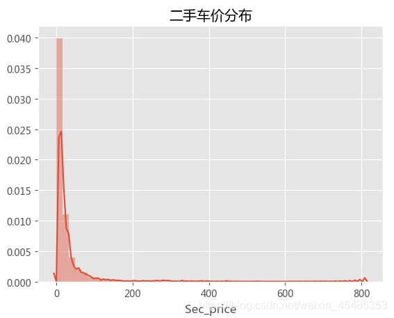
#查看二手价格的分布，二手车价格则增高则二车数量急剧下降，符合偏态分布
sns.distplot(car.Sec_price)
plt.title('二手车价分布')

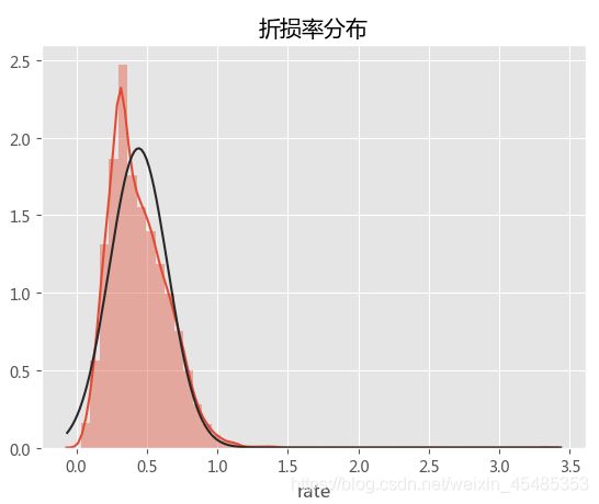
#创造新变量折损率rate（现价/原价）
car['rate']=car.Sec_price.div(car.new_price)
#查看折损率的分布，比较符合正态分布，考虑用折损率来作为作为目标变量
sns.distplot(car.rate,fit=norm)
plt.title('折损率分布')

• 特征筛选，影响二手车价的因素可能有行驶公里km、行驶时间time、品牌Brand、车型款式name等，接下来探索一下各因素与折损率rate之间的关系。

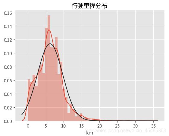
行驶里程km

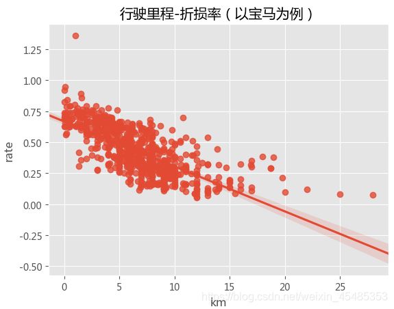
#从分布来看，行驶里程km较符合正态分布，并且与折损率rate间存在明显的负相关（以宝马为例），正常来说，车辆的折损率都是低于1的，（去除rate>1的异常点以及行驶里程超过25km的离散点）    
sns.distplot(car.km,fit=norm)
plt.title('行驶里程-折损率')
sns.regplot('km','rate',data=car[car.Brand=='宝马'])
plt.title('行驶里程-折损率（以宝马为例）')

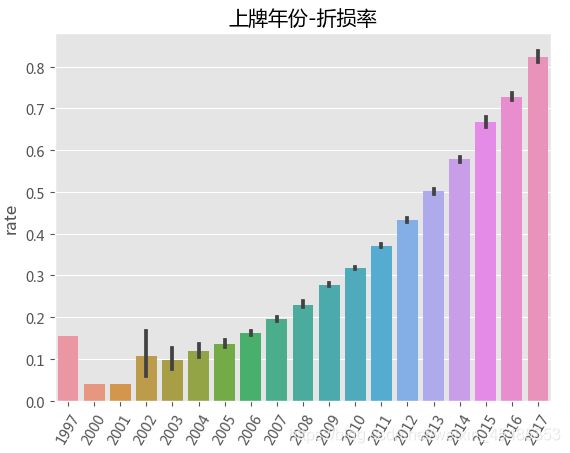
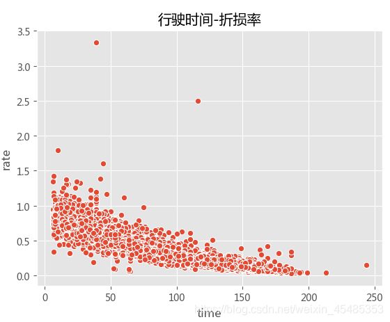
行驶时间time

#行驶时间、上牌年份与折损率呈现负相关性。
sns.barplot('year','rate',data=car)
plt.xticks(rotation=60)
plt.title('上牌年份-折损率')

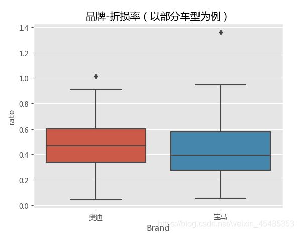
品牌Brand

#Brand与折损率相关，以奥迪，宝马，荣威，名爵为例，不同品牌rate的平均值以及分布不一样，存在异常值。
sns.boxplot('Brand','rate',data=car[car.Brand.isin(['奥迪','宝马'])])
plt.title('品牌-折损率（以部分车型为例）')

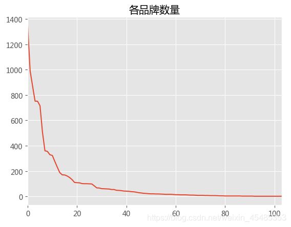
#品牌数目众多，且数量分布不均，部分品牌数量太少不具有代表性，且不利于模型验证（去除少于10辆的车型）    
brand_count=car.Brand.value_counts()
brand_count.index=np.arange(len(brand_count.values))
brand_count.plot()
plt.title('各品牌数量')

去除异常值

#去除异常值，特征筛选
car1=car[(car.rate<1)&(car.km<25)]
car1=car1[~car1.name.isin(['1995','1999','2000','2001','2002'])]
number=dict(zip(car1.groupby('Brand').rate.count().index,car1.groupby('Brand').rate.count().values))
car1['number']=car1.Brand.map(number)
car1=car1.loc[car1.number>=10] 
x=car1[['Brand','km','time','name']]
y=car1['rate'] 

特征编码

#特征Brand和name是类别特征，使用one-hot对变量编码，得到最终数据
x=pd.get_dummies(x)
print(len(x.columns)) #特征维度有71个
71

三、建立模型

划分训练集和测试集

#划分训练集、测试集
xtrain,xtest,ytrain,ytest=train_test_split(x.values,y.values,test_size=.3,random_state=0)
#划分标准化的训练集、测试集
xstd=StandardScaler().fit_transform(x) 
xtrainstd,xteststd,ytrain,ytest=train_test_split(xstd,y.values,test_size=.3,random_state=0)

• 线性回归

#建立线性回归模型
lr=LinearRegression()
lr.fit(xtrain,ytrain)
lrpred=lr.predict(xtest)
lrpredtrain=lr.predict(xtrain)

#R2评估
print(r2_score (ytest,lrpred)) #测试集R2评分
0.8669428574244431
print(r2_score (ytrain,lrpredtrain))#训练集R2评分
0.8594804025897764
#结合交叉验证评估
print(cross_val_score(lr,xtrain,ytrain,cv=5).mean())  
0.8562639774220744

• 调参SVM模型（线性SVR和RBF核函数SVR）

#使用线性SVR模型与非线性SVR模型（RBF核函数）分别进行拟合，SVM模型的输入需要标准化
#线性SVR、调参
svr=LinearSVR()
Cs=[1,10,100,1000,10000]
params={'C':Cs}
gridsvr=GridSearchCV(svr,param_grid=params,cv=5)
gridsvr.fit(xtrainstd,ytrain)
print(gridsvr.best_params_) 
 {'C': 1}
print(gridsvr.best_score_) #训练集结果
0.8297852276978468 
#最优参数模型
svr=LinearSVR(C=1)
svr.fit(xtrainstd,ytrain)
svrpred=svr.predict(xteststd)
print(r2_score (ytest,svrpred))  #测试集R2评分，略低于线性回归
0.8356441749023596

#rbf核非线性SVR、调参
svr_rbf=SVR(kernel='rbf',gamma='auto')
gridsvr_rbf=GridSearchCV(svr_rbf,param_grid=params,cv=5)
gridsvr_rbf.fit(xtrainstd,ytrain)
print(gridsvr_rbf.best_params_)  
 {'C': 10}
print(gridsvr_rbf.best_score_)#训练集结果
0.8622494426824513
#最优参数模型
svr_rbf=SVR(C=10,kernel='rbf',gamma='auto')
svr_rbf.fit(xtrainstd,ytrain)
svrpred2=svr_rbf.predict(xteststd)
print(r2_score (ytest,svrpred2))
0.8752909049370735   #测试集结果，rbf核SVR模型结果比线性SVR更好，略高于线性回归结果

• MLP

#默认参数的MLP回归模型，效果一般
mlpr=MLPRegressor()
mlpr.fit(xtrain,ytrain)
mlppred=mlpr.predict(xtest)
mlppredtrain=mlpr.predict(xtrain)
print(r2_score (ytrain,mlppredtrain))#训练集R2评分
0.8711448569099354
print(r2_score (ytest,mlppred)) #测试集R2评分
0.8648966919561516

• 随机森林

#使用默认参数的随机森林模型，进行拟合
rfr = RandomForestRegressor()
rfr.fit(xtrain,ytrain)
scores =cross_val_score(rfr, xtrain,ytrain, cv=5) #交叉验证得到R2评分
print(scores.mean())
0.8617835669309049
rpred=rfr.predict(xtest)
print(r2_score (ytest,rpred)) #测试集评分，效果优于其他模型
0.8753017649870939

#简单调参，决策树的个数为400时可获得性能略微提升
ns=[200,400,600,800]
gridrfr=GridSearchCV(rfr,param_grid={'n_estimators':ns},scoring='r2',cv=5)
gridrfr.fit(xtrain,ytrain)
print(gridrfr.best_params_)
{'n_estimators': 800}
print(gridrfr.best_score_) #训练集评分
0.8704172423686983
#最佳参数模型
rfr2 = RandomForestRegressor(n_estimators=800)
rfr2.fit(xtrain,ytrain)
rpred2=rfr2.predict(xtest)
print(r2_score (ytest,rpred2)) #测试集评分
0.8858743975574236

• XGBoost

#默认参数的XGBoost模型，是所有模型中拟合最准确的
xgb=XGBRegressor()
xgb.fit(xtrain,ytrain)
xgbpred=xgb.predict(xtest)
xgbpredtrain=xgb.predict(xtrain)
print(r2_score (ytrain,xgbpredtrain))#训练集R2评分
0.8807846709266941
print(r2_score (ytest,xgbpred)) #测试集R2评分
0.8798086358957151

综上，
1，本数据样本数据量相对特征数较多，模型比较简单，也不易出现过拟合情况。
2，运用多种回归模型进行拟合，XGBoost、MLP模型与随机森林模型具有最高的准确率，但相对线性回归、SVR模型区别不是特别大，有限时间空间下，使用简单模型也可以获得不错的效果。
3，对SVM模型与随机森林进行过了简单调参，提高了准确率，可对各模型继续调参优化，获得更好的效果。