pytorch入门：60分钟闪电战-2

神经网络

https://pytorch.org/tutorials/beginner/blitz/neural_networks_tutorial.html

使用torch.nn包构造神经网络。

nn取决于 autograd定义模型并区分它们。一个nn.Module包含层，和一种方法forward(input)，它返回output。

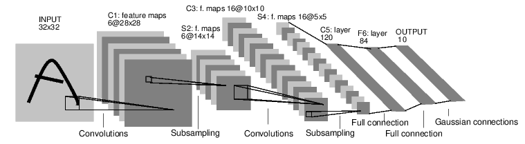
样例convnet是一个简单的前馈网络。它接受输入，一个接一个地通过几个层输入，然后最终给出输出。

前馈神经网络（feedforward neural network），简称前馈网络，是人工神经网络的一种。在此种神经网络中，各神经元从输入层开始，接收前一级输入，并输出到下一级，直至输出层。整个网络中无反馈，可用一个有向无环图表示。

前馈神经网络采用一种单向多层结构。其中每一层包含若干个神经元，同一层的神经元之间没有互相连接，层间信息的传送只沿一个方向进行。其中第一层称为输入层。最后一层为输出层．中间为隐含层，简称隐层。隐层可以是一层。也可以是多层。（参考自百度百科）

神经网络的典型训练程序如下：

• 定义具有一些可学习参数（或权重）的神经网络
• 迭代输入数据集
• 通过网络处理输入
• 计算损失（输出距离正确多远）
• 将渐变传播回网络参数
• 通常使用简单的更新规则更新网络权重： weight = weight - learning_rate * gradient

定义网络

import torch
import torch.nn as nn
import torch.nn.functional as F


class Net(nn.Module):

    def __init__(self):
        super(Net, self).__init__()
        # 1 input image channel, 6 output channels, 3x3 square convolution
        # kernel
        self.conv1 = nn.Conv2d(1, 6, 3)
        self.conv2 = nn.Conv2d(6, 16, 3)
        # an affine operation: y = Wx + b
        self.fc1 = nn.Linear(16 * 6 * 6, 120)  # 6*6 from image dimension
        self.fc2 = nn.Linear(120, 84)
        self.fc3 = nn.Linear(84, 10)

    def forward(self, x):
        # Max pooling over a (2, 2) window
        x = F.max_pool2d(F.relu(self.conv1(x)), (2, 2))
        # If the size is a square you can only specify a single number
        x = F.max_pool2d(F.relu(self.conv2(x)), 2)
        x = x.view(-1, self.num_flat_features(x))
        x = F.relu(self.fc1(x))
        x = F.relu(self.fc2(x))
        x = self.fc3(x)
        return x

    def num_flat_features(self, x):
        size = x.size()[1:]  # all dimensions except the batch dimension
        num_features = 1
        for s in size:
            num_features *= s
        return num_features


net = Net()
print(net)

输出：

Net(
  (conv1): Conv2d(1, 6, kernel_size=(3, 3), stride=(1, 1))
  (conv2): Conv2d(6, 16, kernel_size=(3, 3), stride=(1, 1))
  (fc1): Linear(in_features=576, out_features=120, bias=True)
  (fc2): Linear(in_features=120, out_features=84, bias=True)
  (fc3): Linear(in_features=84, out_features=10, bias=True)
)

可以看到这里我们定义了如下结构的网络：

卷积层1：1通道输入，6通道输出（输入通道输出通道时可以根据自己的需求来制定的），核大小为3*3的网络，步长为1，padding未指定应当默认为0.

卷积层2：接受卷积层1的输出，因此6通道输入，16通道输出，核大小和步长不改变

三个全连接层，在输出结果中通过in和out可以看到内在的联系。

只需定义forward函数，backward 自动定义函数（计算渐变的位置）autograd。可以在forward函数中使用任何Tensor操作。

模型的可学习参数由 net.parameters()返回。

params = list(net.parameters())
print(len(params))
print(params[0].size())  # conv1's .weight


输出：

10
torch.Size([6, 1, 3, 3])

让我们尝试一个随机的32x32输入。注意：此网络（LeNet https://www.jiqizhixin.com/graph/technologies/6c9baf12-1a32-4c53-8217-8c9f69bd011b）的预期输入大小为32x32。

input = torch.randn(1, 1, 32, 32)
out = net(input)
print(out)

输出：

tensor([[-0.0776,  0.0463,  0.1200,  0.0808,  0.0915, -0.1071, -0.0830,  0.0332, -0.0552, -0.0365]], grad_fn=)

补充：N=(W-F+2P)/S+1 参考：https://blog.csdn.net/sinat_42239797/article/details/90646935
其中N：输出大小
W：输入大小
F：卷积核大小
P：填充值的大小
S：步长大小

在这个网络中卷积层1的输出N=（32-3+0）/1+1=30，注意文章最开始的LeNet示意图使用的是5*5的卷积核得到结果为28。

卷积层2（30-3+0）/1+1=28

使用随机梯度将所有参数和反向的梯度缓冲区归零：

net.zero_grad()
out.backward(torch.randn(1, 10))

注意：

torch.nn仅支持迷你批次。整个torch.nn 软件包仅支持小批量样本的输入，而不是单个样本。

例如，nn.Conv2d将采用4D Tensor of 。nSamples x nChannels x Height x Width

如果有一个样本，只需使用input.unsqueeze(0)添加假批量维度。

损失函数

损失函数采用（输出，目标）输入对，并计算估计输出距目标的距离的值。

nn包下有几种不同的 损失函数。一个简单的损失是：nn.MSELoss它计算输入和目标之间的均方误差。

例如：

output = net(input)
target = torch.randn(10)  # a dummy target, for example
target = target.view(1, -1)  # make it the same shape as output
criterion = nn.MSELoss()

loss = criterion(output, target)
print(loss)

如果按照loss向后方向，使用其 .grad_fn属性，您将看到如下所示的计算图：

input -> conv2d -> relu -> maxpool2d -> conv2d -> relu -> maxpool2d
      -> view -> linear -> relu -> linear -> relu -> linear
      -> MSELoss
      -> loss

因此，当我们调用时loss.backward()，整个图形会随着损失而区分，并且图形中的所有张量都requires_grad=True 将.grad使用渐变累积其Tensor。

print(loss.grad_fn)  # MSELoss
print(loss.grad_fn.next_functions[0][0])  # Linear
print(loss.grad_fn.next_functions[0][0].next_functions[0][0])  # ReLU

输出（loss，MSEloss，LInear，ReLU）

tensor(1.6761, grad_fn=)

 

Backprop

loss.backward()得到反向传播错误。需要清除现有渐变，否则渐变将累积到现有渐变。

调用loss.backward()，看一下conv1在向后之前和之后的偏差梯度。（在保留前文input以及loss的基础上）

net.zero_grad()     # zeroes the gradient buffers of all parameters

print('conv1.bias.grad before backward')
print(net.conv1.bias.grad)

loss.backward()

print('conv1.bias.grad after backward')
print(net.conv1.bias.grad)

输出：

conv1.bias.grad before backward
None    //在示例中为tensor([0., 0., 0., 0., 0., 0.])
conv1.bias.grad after backward
tensor([ 0.0092,  0.0036,  0.0003,  0.0014, -0.0048,  0.0015])

 

更新权重

实践中使用的最简单的更新规则是随机梯度下降（SGD）：

weight = weight - learning_rate * gradient

我们可以使用简单的python代码实现它：

learning_rate = 0.01
for f in net.parameters():
    f.data.sub_(f.grad.data * learning_rate)

但是，当使用神经网络时，希望使用各种不同的更新规则，例如SGD，Nesterov-SGD，Adam，RMSProp等。为了实现这一点，我们构建了一个小包：torch.optim，它实现了所有这些方法。使用它非常简单：

import torch.optim as optim

# create your optimizer
optimizer = optim.SGD(net.parameters(), lr=0.01)

# in your training loop:
optimizer.zero_grad()   # zero the gradient buffers使用手动将梯度缓冲区设置为零 optimizer.zero_grad()因为渐变是按Backprop部分中的说明累积的。
output = net(input)
loss = criterion(output, target)
loss.backward()
optimizer.step()    # Does the update