Understanding Hough Transform With Python硬核翻译~

 

Hough变换（Duda和Hart，1972），最初是一种检测图像中线条的技术，现在主要被用来检测2D和3D曲线。

该文主要从以下两方面进行解析

1.如何工作的 ？

- 渐变 - 截距参数空间

笛卡尔形式的线有以下等式：

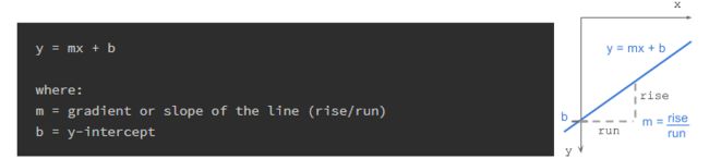
gradient or slope of the line (rise/run) 

线的梯度或斜率（上升/下降）

b = y-intercept

b = y-截距

给定一组边缘点或指示边缘的二进制图像，我们希望找到在图像空间中连接这些点的尽可能多的线。

假设我们有2个边缘点（x1，y1）和（x2，y2）。对于各种梯度值（m = -0.5,1.0,1.5等）的每个边缘点，我们计算相应的b值。下图显示了通过图像空间中的边缘点的各种线以及这些线在参数空间中的图。在笛卡尔图像空间中共线的点将在m-b参数空间中的点处相交。

图像空间中一条线上的所有点都在参数空间中的公共点处相交。该公共点（m，b）表示图像空间中的线。

不幸的是，当线是垂直的时，斜率m是未定义的（除以0！）。
为了克服这个问题，我们使用了另一个参数空间，即霍夫空间。

2.它是如何工作的 - 角度-距离参数空间
极坐标系中的线具有以下等式：

ρ (rho) =从原点到直线的距离。 [-max_dist到max_dist]。 max_dist是图像的对角线长度。

θ =从原点到直线的角度。 [-90°至90°]

如果你对ρ的派生方式感兴趣，我已经在最底层的附加部分列出了数学：导出rho。

为了解释霍夫变换，我将使用一个简单的例子。 我已经创建了一个大小为30 x 30像素的输入二进制图像，其中点（5,25）和（20,10）如下所示。 通过用-90∘到90∘的每个角度的点计算ρ，将图像变换到霍夫空间（负角度从原点水平逆时针开始，正角度是顺时针方向）。 霍夫空间中的点形成正弦曲线。

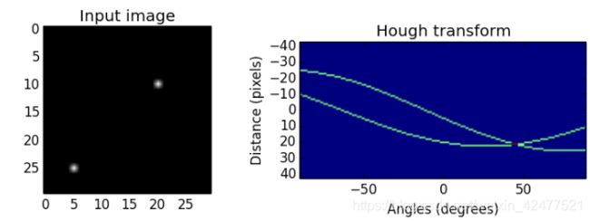
两个边缘点在不同角度的ρ值： 

我们看到霍夫空间中的曲线在45°处相交，ρ= 21。
由图像空间中的共线点生成的曲线在霍夫变换空间中的峰（ρ，θ）中相交。 曲线在一点处相交越多，图像空间中的线条将获得的“vote”越多。 我们将在下一个实现部分中看到这一点。 

 

算法步骤
1.拐角或边缘检测。 （例如，使用canny，sobel，自适应阈值处理）。得到的二进制/灰度图像将具有指示非边缘的0和指示边缘的1或以上。这是我们的输入图像。
2.Rho范围和Theta范围创建。 ρ的范围从-max_dist到max_dist，其中max_dist是输入图像的对角线长度。 θ的范围为-90∘至90∘。您可以在范围内使用更多或更少的箱柜来权衡准确性，空间和速度。例如。每隔三个角度在-90∘到90∘之间，从180减少到60。
3.θ对ρ的Hough累加器。它是一个2D数组，其行数等于ρ值的数量，列数等于θ值的数量。
4.在累加器中投票。对于每个边缘点和每个θ值，找到最接近的ρ值并在累加器中递增该索引。每个元素告诉有多少点/像素为具有参数（ρ，θ）的潜在线候选者贡献“投票”。
5.高峰发现。累加器中的局部最大值表示输入图像中最突出的线的参数。通过应用阈值或相对阈值（等于或大于全局最大值的某个固定百分比的值），可以最容易地找到峰值。 

代码实现：

import numpy as np
import imageio
import math

def rgb2gray(rgb):
    return np.dot(rgb[..., :3], [0.299, 0.587, 0.114]).astype(np.uint8)


def hough_line(img, angle_step=1, lines_are_white=True, value_threshold=5):
    """
    Hough transform for lines
    Input:
    img - 2D binary image with nonzeros representing edges
    angle_step - Spacing between angles to use every n-th angle
                 between -90 and 90 degrees. Default step is 1.
    lines_are_white - boolean indicating whether lines to be detected are white
    value_threshold - Pixel values above or below the value_threshold are edges
    Returns:
    accumulator - 2D array of the hough transform accumulator
    theta - array of angles used in computation, in radians.
    rhos - array of rho values. Max size is 2 times the diagonal
           distance of the input image.
    """
    # Rho and Theta ranges
    thetas = np.deg2rad(np.arange(-90.0, 90.0, angle_step))
    width, height = img.shape
    diag_len = int(round(math.sqrt(width * width + height * height)))
    rhos = np.linspace(-diag_len, diag_len, diag_len * 2)

    # Cache some resuable values
    cos_t = np.cos(thetas)
    sin_t = np.sin(thetas)
    num_thetas = len(thetas)

    # Hough accumulator array of theta vs rho
    accumulator = np.zeros((2 * diag_len, num_thetas), dtype=np.uint8)
    # (row, col) indexes to edges
    are_edges = img > value_threshold if lines_are_white else img < value_threshold
    y_idxs, x_idxs = np.nonzero(are_edges)

    # Vote in the hough accumulator
    for i in range(len(x_idxs)):
        x = x_idxs[i]
        y = y_idxs[i]

        for t_idx in range(num_thetas):
            # Calculate rho. diag_len is added for a positive index
            rho = diag_len + int(round(x * cos_t[t_idx] + y * sin_t[t_idx]))
            accumulator[rho, t_idx] += 1

    return accumulator, thetas, rhos


def show_hough_line(img, accumulator, thetas, rhos, save_path=None):
    import matplotlib.pyplot as plt

    fig, ax = plt.subplots(1, 2, figsize=(10, 10))

    ax[0].imshow(img, cmap=plt.cm.gray)
    ax[0].set_title('Input image')
    ax[0].axis('image')

    ax[1].imshow(
        accumulator, cmap='jet',
        extent=[np.rad2deg(thetas[-1]), np.rad2deg(thetas[0]), rhos[-1], rhos[0]])
    ax[1].set_aspect('equal', adjustable='box')
    ax[1].set_title('Hough transform')
    ax[1].set_xlabel('Angles (degrees)')
    ax[1].set_ylabel('Distance (pixels)')
    ax[1].axis('image')

    # plt.axis('off')
    if save_path is not None:
        plt.savefig(save_path, bbox_inches='tight')
    plt.show()


if __name__ == '__main__':
    imgpath = 'imgs/binary_crosses.png'
    img = imageio.imread(imgpath)
    if img.ndim == 3:
        img = rgb2gray(img)
    accumulator, thetas, rhos = hough_line(img)
    show_hough_line(img, accumulator, save_path='imgs/output.png')

扩展

Hough变换可以被检测圆方程扩展，。

此外，它可以推广到检测任意形状（D. H. Ballard，1981）。

另一种方法是Progressive Probabilistic Hough变换（Galamhos等，1999）。 该算法在累加器中使用投票点的随机子集，并检查具有最小间隙的最长像素段。 超出最小长度阈值的线段将添加到列表中。 这将返回图像中每个线段的起点和终点。 它有3个阈值：Hough累加器中的最小投票数，合并的最大行间距和最小行长度。

Extras

Deriving rho: ρ = x cos θ + y sin θ

使用基本的三角学，我们知道对于直角三角形，

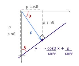
我们希望将参数（m，b）的笛卡尔形式y = mx + b转换为带参数（ρ，θ）的极坐标形式。

来自距离ρ的原点的线具有的梯度。 与其垂直的感兴趣线将具有的负倒数梯度值。 对于b，感兴趣线的y轴截距，。

在且的情况下，得到。

 

 

实际应用

First, we need to read in an image:

import matplotlib.pyplot as pltimport matplotlib.image as mpimg

image = mpimg.imread('exit-ramp.jpg')

plt.imshow(image)

Here we have an image of the road, and it's fairly obvious by eye where the lane lines are, but what about using computer vision?

Let's go ahead and convert to grayscale.

import cv2  #bringing in OpenCV libraries

gray = cv2.cvtColor(image, cv2.COLOR_RGB2GRAY) #grayscale conversion

plt.imshow(gray, cmap='gray')

Let’s try our Canny edge detector on this image. This is where OpenCV gets useful. First, we'll have a look at the parameters for the OpenCV Canny function. You will call it like this:

edges = cv2.Canny(gray, low_threshold, high_threshold)

In this case, you are applying Canny to the image gray and your output will be another image called edges.low_threshold and high_threshold are your thresholds for edge detection.

The algorithm will first detect strong edge (strong gradient) pixels above the high_threshold, and reject pixels below the low_threshold. Next, pixels with values between the low_threshold and high_threshold will be included as long as they are connected to strong edges. The output edges is a binary image with white pixels tracing out the detected edges and black everywhere else. See the OpenCV Canny Docs for more details.

What would make sense as a reasonable range for these parameters? In our case, converting to grayscale has left us with an 8-bit image, so each pixel can take 2^8 = 256 possible values. Hence, the pixel values range from 0 to 255.

This range implies that derivatives (essentially, the value differences from pixel to pixel) will be on the scale of tens or hundreds. So, a reasonable range for your threshold parameters would also be in the tens to hundreds.

As far as a ratio of low_threshold to high_threshold, John Canny himself recommended a low to high ratio of 1:2 or 1:3.

We'll also include Gaussian smoothing, before running Canny, which is essentially a way of suppressing noise and spurious gradients by averaging (check out the OpenCV docs for GaussianBlur). cv2.Canny() actually applies Gaussian smoothing internally, but we include it here because you can get a different result by applying further smoothing (and it's not a changeable parameter within cv2.Canny()!).

You can choose the kernel_size for Gaussian smoothing to be any odd number. A larger kernel_size implies averaging, or smoothing, over a larger area. The example in the previous lesson was kernel_size = 3.

Note: If this is all sounding complicated and new to you, don't worry! We're moving pretty fast through the material here, because for now we just want you to be able to use these tools. If you would like to dive into the math underpinning these functions, please check out the free Udacity course, Intro to Computer Vision, where the third lesson covers Gaussian filters and the sixth and seventh lessons cover edge detection.

#doing all the relevant imports

import matplotlib.pyplot as plt

import matplotlib.image as mpimg

import numpy as npimport cv2

# Read in the image and convert to grayscale

image = mpimg.imread('exit-ramp.jpg')

gray = cv2.cvtColor(image, cv2.COLOR_RGB2GRAY)

# Define a kernel size for Gaussian smoothing / blurring# Note: this step is optional as cv2.Canny() applies a 5x5 Gaussian internally

kernel_size = 3

blur_gray = cv2.GaussianBlur(gray,(kernel_size, kernel_size), 0)

# Define parameters for Canny and run it# NOTE: if you try running this code you might want to change these!

low_threshold = 1

high_threshold = 10

edges = cv2.Canny(blur_gray, low_threshold, high_threshold)

# Display the image

plt.imshow(edges, cmap='Greys_r')

Here I've called the OpenCV function Canny on a Gaussian-smoothed grayscaled image called blur_gray and detected edges with thresholds on the gradient of high_threshold, and low_threshold.

In the next quiz you'll get to try this on your own and mess around with the parameters for the Gaussian smoothing and Canny Edge Detection to optimize for detecting the lane lines and not a lot of other stuff.